Gold Price Relative Return Prediction with Machine Learning

Models

Runjie Zhang

Woodsworth College, University of Toronto, Toronto, Canada

Keywords: Gold Price,Relative Return Prediction, Machine Learning Models.

Abstract: Gold is a safe haven asset during the crisis; it can help investors to hedge against inflation and economic

uncertainty. Thus, predicting gold return is essential for financial institutions and individual investors. This

paper uses Extreme Gradient Boosting (XGBoost), Support Vector Regression (SVR) and Random Forest

(RF) model to predict gold return—dataset sources from Yahoo Finance. Features of oil price, volatility index,

S&P 500 index, and USD index are add-ed for better prediction. Technical features such as MACD difference,

RSI, and Bollinger%B are applied for better accuracy. To find the best parameters, grid search is conducted.

To eval-uate the model's performance, mean square error, root mean square error, mean absolute error, R-

squared (R2) value, and trend accuracy are calculated and compared among models. RF and SVR give an R2

value of 0.79, and XGBoost gives an R2 value of 0.72. The overall perfor-mance of the SVR and RF models

is nearly the same, but the RF model has higher trend accu-racy and better prediction fitness. The SVR model

performs much better in predicting extreme values than RF.

1 INTRODUCTION

Countries' central banks hold gold reserves as a

guarantee to pay for trade on the world market

(Makala & Li, 2021). It makes gold a key asset for

investors who seek stability. Recently, geo-political

risk and economic uncertainties have existed more

often than before. Predicting gold's relative return

accurately can help investors and institutions make

better decisions and manage their risks.

Basher et al. use RF and logit models to predict

Bitcoin and gold price direction. The paper mentions

that the most influential features for prediction are the

MACD signal, oil volatility index, and bond yields.

These features are related to what will be applied in

this paper. The re-sult shows that RFs are effective

for predicting gold price direction with technical

indicators (Basher & Sadorsky, 2022).

Jayendrakamesh et al. compare linear regression

and RF to predict gold prices. It uses the currency

exchange rate as a feature and gets a result that RF

gives a better result. Instead of gold price prediction,

this paper will focus on relative gold returns

(Jayendrakamesh et al., 2024).

Jabeur et al. use linear regression, neural

networks, RF, and XGBoost to predict gold prices. It

uses Shapley's Additive explanation method and finds

that silver price, inflation, and other macroeconomic

factors significantly influence gold prices. The study

concluded that gradient-boosting methods give a

better result (Jabeur et al., 2024).

This paper extends empirical work on gold

relative return prediction by using new strongly

correlated variables such as the WTI oil prices, the

VIX index, the SP500, and the USD index. Technical

indicators such as Bollinger Bands, MACD, and RSI

are also applied as features to make forecasts more

accurate and improve the model. The paper will apply

three machine learning models: SVR, RF, and

XGBoost. The performance of three different models

will be compared. Instead of only using historical

gold price data to predict future relative returns, this

paper aims to use more related variables and technical

features to make prediction more accurate. Finally,

this paper aims to find models that can accurately and

effectively predict gold return based on available data

or technical features.

Zhang and R.

Gold Price Relative Return Prediction with Machine Learning Models.

DOI: 10.5220/0013528700004619

In Proceedings of the 2nd International Conference on Data Analysis and Machine Learning (DAML 2024), pages 579-584

ISBN: 978-989-758-754-2

579

2 DATA AND METHOD

2.1 Data collection and description

Data is collected from Yahoo Finance. The dataset

contains eight variables and 5849 observa-tions. Date

is the record date. Data contains date from 2000-8-30

to 2023-12-29. The date without the gold trade is not

included. Variable Open is the open price of gold on

that date. High and Low are the highest and lowest

prices of gold that date. Close is the difference be-

tween the gold price on the current date and the last

day. SP500_Close is the S&P 500 index close point

that date. The index is one of the most crucial stock

indices in United States. It represents the performance

of the best 500 stocks in the American stock market.

USD_Index_Close is the United States Dollar index

close point that date. It can represent overall power

against other primary currencies worldwide.

vix_data_Close is the volatility in-dex. It can

represent the geopolitical and economic risk or

uncertainty level in the market. WTI_Crude is the oil

price of West Texas Intermediate. It is the critical

global oil price stand-ard.

Gold and WTI crude oil are indirectly linked

through inflation (Jain & Biswal, 2016). Oil and gold

prices have shown a positive correlation. The USD

index reflects the value of the dol-lar, which will

directly impact the price of gold. Investors may find

other assets instead of the US dollar to preserve value

when the US dollar becomes weaker. Gold is a

traditional safe-haven asset. Thus, gold will attract

more investors when USD becomes weaker, and the

in-creasing demand will make the gold price higher.

Similarly, because of the safe characteristics of gold,

when the VIX index increases, which indicates that

the risk becomes higher. Inves-tors need to invest on

gold to hedge the risk (Hapau, 2023). S&P500

reflects the risk senti-ment and capital allocation.

When the stock market is in a bull market period,

people tend to allocate more money to the stock

market for high returns. Thus, less money is willing

to allo-cate to gold. Conversely, if the stock market is

experiencing a downturn, more people will be willing

to buy gold to avoid high risk in the stock market (Jain

& Biswal, 2016).

2.2 Data processing and freature

creation

To ensure stationarity, model stability, and accuracy,

this paper will use the relative return of gold instead

of the gold close price directly (absolute return). As

shown in formula (1), relative returns are calculated

as the percentage change between the current gold

price and the gold price the previous day. P_t

represents the price of gold today and P_(t-1)

represents the price of gold on the last day.

Return =



−P







Three features are created to predict gold return

better. Moving average convergence diver-gence

(MACD) difference is used as an indicator to measure

the momentum and trend strength of gold price.

Formulas (2), (3), (4), (5) show how to calculate the

MACD difference. The MACD difference is

calculated by the difference between the MACD line

and signal line. The MACD line is calculated by

subtracting the 26-day exponential moving average

(EMA) from the 12-day. The signal line is the 9-day

EMA of the MACD line. where P is the gold price for

the period, i is the current period, n – number of data

considered for the calculation of the moving average

(Aguirre et al., 2020).

EMA = P



∗

n+1

+EMA



∗1−

n+1





MACD line = EMA



−EMA







Signal line = EMA







MACD difference = MACD line − Signal line





The relative strength index (RSI) is an indicator

that can identify overbought or oversold in the

market. It measures the speed of change of price

movements. Formulas (6), (7), (8), (9) (10) show how

to calculate RSI. The first step is to calculate the price

change. The second step is to calculate average gains

(AG) and losses (AL), n, which is the look-back

period of 14 days. The third step is to calculate

relative strength. Finally, relative strength is used to

calculate the RSI. When the RSI value exceeds 70, an

overbought signal exists on the asset. When the RSI

value is lower than 30, an oversold signal exists on

the asset (Husaini et al., 2024). P_t represents the

price of gold today and P



represents the price of

gold on the last day.

∆P



−P







AG =

∑

∆P





∆P









AL =

∑|

∆P



|

∆P









RS =





DAML 2024 - International Conference on Data Analysis and Machine Learning

580

RSI = 100 − 

100

1+RS







Bollinger %B (%B) is an indicator that helps

investors notice the volatility and potential price

reversal. Formulas (11), (12) and (13) show how to

calculate %B. The first step is calcu-lating the 20-day

moving average (MA) and setting it as the middle

band. The second step is calculating the upper and

lower Bollinger band (UB LB). Finally, use the

current price, as well as the upper and lower Bollinger

bands, to get Bollinger %B. When %B is higher than

one or lower than one, a signal of high volatility and

potential trend reversal may appear.

UB = MA



+2std





LB = MA



−2std





%B =



−LB

UB − LB





Table 1 shows the information of created features.

As features require past data to calculate, the first few

rows of data contain missing values. Table 2 shows

the cleaned data after dealing with all missing values.

The dataset contains 11 variables and 5802

observations.

Table 1: Input Features information.

MACD_Diff Bollinger_%B RSI

Mean 0.011 0.55 50.03

Standard

devia-

tion(std)

4.32 0.33 4.97

Min -29.19 -0.45 28.37

25% -1.95 0.28 47.18

50% 0.13 0.56 50.03

75% 2.12 0.82 52.86

Max 16.77 1.45 73.93

2.3 Model

SVR is a regression model that can find a hyperplane

that best fits the data points. It uses the kernel trick to

transform non-linear relationships to a higher-

dimensional space and fit a hy-perplane efficiently

(Guo et al., 2024).

RF is an ensemble learning method that improves

the traditional decision tree method by combining

multiple trees and output the average value of

different trees to reduce variance and improve

prediction accuracy. It uses different bootstrapped

samples and only considers a random subset of

predictors at each split (Basher & Sadorsky, 2022).

XGBoost is an advanced gradient-boosting

algorithm that sequentially builds an ensemble of

decision trees. Each tree corrects the error made by

the previous tree (Suryana & Sen, 2021).

3 RESULTS AND DISCUSSION

3.1 Experiment and parameters

SVR, RF, and XGBoost models are trained based on

80% of the dataset's data, which are ran-domly

chosen. The remaining 20% of data is assigned to be

test data for validation. Grid search is applied to find

the best parameters for the models. Before conducting

SVR, a stand-ard scalar is applied to the data.

For SVR, the kernel is compared between radial

basis function (RBF) and linear, the regu-larization

parameter c is compared between 1, 50, and 500, and

the kernel coefficient gamma is compared between

0.001, 0.01, and 0.1. Epsilon, which defines the width

of the epsilon tube, is compared between 0.1, 0.2, and

0.5. The grid search results indicate that RBF, c

equals 50, gamma equals 0.01, and epsilon equals 0.2

gives the best result.

Table 2: This caption has more than one line so it has to be set to justify.

Close Open High Low vix WTI SP500 USD_Index

Mean 0.00042 0.00042 0.00041 0.00041 0.0025 -0.00016 0.00029 -0.00001

Std 0.011 0.011 0.10 0.11 0.075 0.051 0.012 0.0049

25% -0.0048 -0.0050 -0.0046 -0.0045 -0.30 -3.06 -0.12 -0.027

50% 0.00046 0.00038 0.00016 0.00075 -0.0058 0.0011 0.00063 0

75% 0.00062 0.0061 0.0057 0.0057 0.034 0.014 0.0059 0.0028

Max 0.090 0.12 0.13 0.069 1.16 0.38 0.12 0.026

Gold Price Relative Return Prediction with Machine Learning Models

581

For RF, a number of parameters set in the decision

tree is compared among 100, 200, and 300, the

maximum depth of each decision tree is compared

among 5, 8, and 10, and the min-imum sample leaf is

compared between 1 and 5. The gird search result

indicates that the number of parameters set equals

200, the maximum depth of each decision tree equals

10, the minimum sample leaf equals 1, and the

algorithm considers the square root of a total number

of features to give the best result.

For XGBoost, fraction of features to be randomly

sample for each tree (colsample by tree) is compared

among 0.5, 0.7 and 0.8. The maximum depth of each

tree is compared among 10, 15 and 20. The learning

rate controls the contribution of each tree to the final

model; it is compared between 0.01, 0.05, and 0.1.

Hyperparameter alpha is compared between 1,5, and

10. The result of grid search indicates that colsample

by tree equals 0.5, maximum depth equals 10,

learning rate equals 0.1 and number of estimators

equal to 300 gives the best result.

3.2 Experiment Results

Tables 3 and 4 show the experiment results. For SVR,

a standard scaler is applied. To make the errors of the

three models comparable, inverse transformation is

applied, and errors are calculated based on the new

transformed data.

Table 3: Result of three models.

MSE RMSE MAE R

RF Train 1.31e-05 0.0036 0.0026690 0.89

RF Test 2.36e-05 0.0049 0.0032876 0.79

XGBoost

Train

3.38e-05 0.0058 0.0037 0.73

XGBoost

Test

2.98e-05 0.0055 0.0038 0.72

SVR

Train

1.92e-05 0.0044 0.0030 0.84

SVR

Test

2.21e-05 0.0047 0.0033 0.79

Table 4: Comparison of trend accuracy.

RF XGBoost SVR

Trend

Accurac

0.88 0.85345 0.86

Trend accuracy is calculated as the proportion of

corrected increasing or decreasing trend prediction.

The RF model performs the best; its trend accuracy is

2.2% higher than that of the SVR model.

For train data, the RF model's MSE, RMSE, and

MAE are much lower than those of XGBoost and

SVR, and R2 is much higher in the RF model than in

the other two. This indi-cates that the RF performs

better with the training data and creates less error.

Also, a higher R2 value indicates that RF performs

better at capturing the variance in training data.

For test data, XGboost model performs the worst.

RF and SVR have nearly the same MSE, RMSE,

MAE, and R2. Compared to SVR model, RF model

has slightly lower MSE, slightly higher R2 and

RMSE.

For XGBoost, train data has higher MSE and

RMSE than test data, indicating that training data

undergoes underfitting. Noisy training data may

cause this problem. Conversely, RF and SVR has

much higher value for train data than for test data.

This indicates that the train data of the RF model

undergoes an overfitting problem. The R2 difference

between train data and test of RF is around 0.1 which

is much higher than the 0.054 of SVR. This indicates

that RF has a more vital overfitting problem than

SVR.

From Figure 1, RF predicted value fits the actual

value well, but slight deviation still exists. The

deviation of RF model to predict extreme high value

is big.

From Figure 2, XGBoost fits the actual value but

is worse than RF. Also, XGBoost shows a slightly

delayed response. This indicates that models perform

worse on sudden increases and decreases in gold

return. Also, the performance of XGBoost to predict

extreme high values is even worse than that of the RF

model.

Figure 3 shows that the fitness of the SVR

predicted value is slightly lower than that of RF but

higher than that of SGBoost. For extreme values, the

performance of the SVR model is much better than

that of the other two models.

DAML 2024 - International Conference on Data Analysis and Machine Learning

582

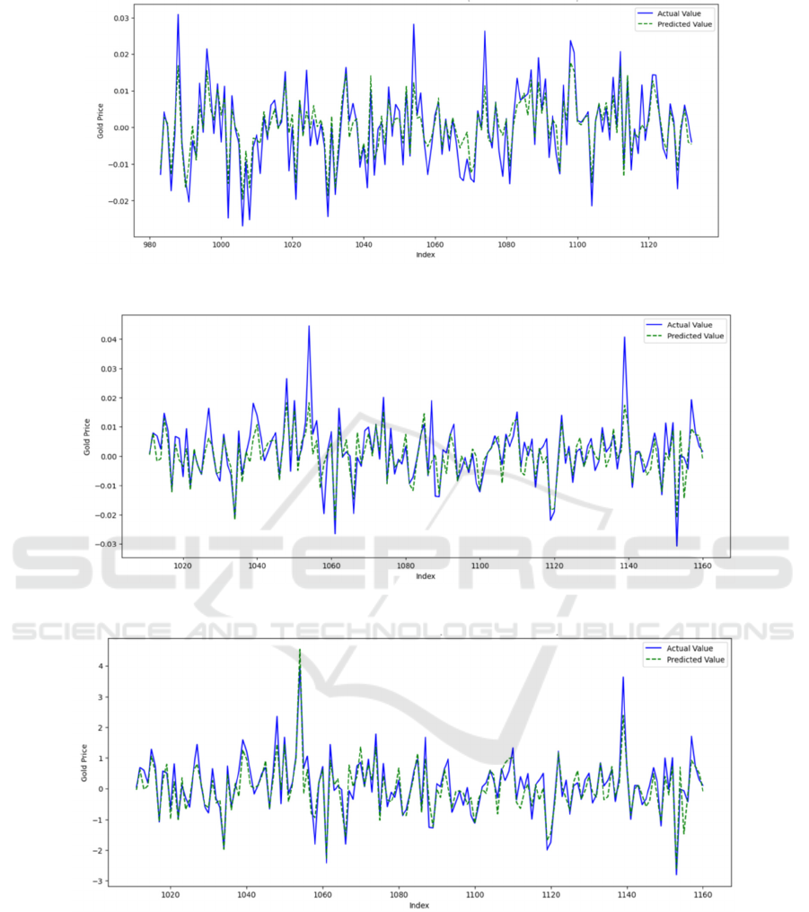
Figure 1: RF Actual vs Predicted gold return (Last 150 test data points) (Photo/Picture credit: Original).

Figure 2: XGBoost Actual vs Predicted gold return (Last 150 test data points) (Photo/Picture credit: Original).

Figure 3. SVR Actual vs Predicted gold return (Last 150 test data points) (Photo/Picture cred-it: Original).

4 CONCLUSIONS

In conclusion, the gold return prediction is

sophisticated but worth researching. For any fi-

nancial institution or individual investor, gold return

is essential. Gold returns can represent the gold price

and reveal the extent of volatility and market

sentiment. By better predicting the gold return,

investors can find more opportunities for other

financial assets. This paper use RF, SVR and

XGBoost to predict gold returns effectively. RF and

SVR give an R2 value of 0.79, and XGBoost gives an

R2 value of 0.72. RF and SVR models have similar

Gold Price Relative Return Prediction with Machine Learning Models

583

errors and R2 values. RF model has better overall

fitness and higher trend prediction accuracy, but SVR

per-forms better at predicting extreme values and has

fewer problems with overfitting. Overall, the RF and

SVR models can both predict gold returns effectively

and accurately. Models still have some limitations.

For XGBoost, the higher train error indicates the

underfitting of training da-ta. For RF and SVR

models, the higher test error than train data indicates

the overfitting of test data.

REFERENCES

Aguirre, A. A. A., Medina, R. A. R., & Méndez, N. D. D.

2020. Machine learning applied in the stock market

through the Moving Average Convergence Divergence

(MACD) indicator. Investment Management &

Financial Innovations, 17(4), 44.

Basher, S. A., & Sadorsky, P. 2022. Forecasting Bitcoin

price direction with random forests: How important are

interest rates, inflation, and market volatility?. Machine

Learning with Applica-tions, 9, 100355.

Guo, Y., Li, C., Wang, X., & Duan, Y. 2024. Gold Price

Prediction Using Two-layer Decomposition and

XGboost Optimized by the Whale Optimization

Algorithm. Computational Economics, 1-33.

Hapau, R. G. 2023. Capital Market Volatility During

Crises: Oil Price Insights, VIX Index, and Gold Price

Analysis. Management & Marketing, 18(3), 290-314.

Husaini, N. A., Gan, Y. J., Ghazali, R., Hassim, Y. M. M.,

Shen Yeap, J., & Joseph, J. S. 2024. Predic-tive

Modeling of Gold Prices: Integrating Technical

Indicators for Enhanced Accuracy. In Inter-national

Conference on Soft Computing and Data Mining (pp.

390-399). Cham: Springer Nature Switzerland.

Jabeur, S. B., Mefteh-Wali, S., & Viviani, J. L. 2024.

Forecasting gold price with the XGBoost algo-rithm

and SHAP interaction values. Annals of Operations

Research, 334(1), 679-699.

Jain, A., & Biswal, P. C. 2016. Dynamic linkages among

oil price, gold price, exchange rate, and stock market in

India. Resources Policy, 49, 179-185.

Jayendrakamesh, S., Michaelraj, T. F., & Yong, L. C. 2024.

Comparing the accuracy of gold price prediction using

linear regression and random forest regression

algorithms for investment. In AIP Conference

Proceedings (Vol. 3161, No. 1). AIP Publishing.

Makala, D., & Li, Z. 2021. Prediction of gold price with

ARIMA and SVM. In Journal of Physics: Conference

Series (Vol. 1767, No. 1, p. 012022). IOP Publishing.

Suryana, Y., & Sen, T. W. 2021. The prediction of gold

price movement by comparing naive bayes, support

vector machine, and K-NN. JISA (Jurnal Informatika

dan Sains), 4(2), 112-120.

DAML 2024 - International Conference on Data Analysis and Machine Learning

584