Train Recurrent Neural Network to Predict Stock Prices Using Daily
Return Rate
Kangrong Shi
School of Information Science and Technology, Beijing University of Technology, Beijing, China
Keywords: Stock Price Prediction, Daily Return, Recurrent Neural Network (RNN), Long Short-Term Memory Network
(LSTM), Gated Recurrent Unit (GRU).
Abstract: In financial markets, where stock prices are extremely volatile, predicting their future movements has always
been a major challenge for the financial and academic communities. This study aims to explore a novel
method of stock market price prediction, that is, using daily returns as training data, to replace the traditional
forecasting models that rely on closing prices. Traditional forecasting models often fail to fully capture the
complex patterns and nonlinear relationships of stock price dynamics, resulting in limited forecasting
accuracy. In order to overcome these limitations, this study uses three advanced models in deep learning:
Recurrent Neural Network (RNN), Long Short-Term Memory Network (LSTM), and Gated Recurrent Unit
(GRU) to improve the accuracy of prediction through daily return data. Three key metrics were used in this
experiment: Root Mean Square Error (RMSE), Mean Absolute Error (MAE), and Mean Square Error (MSE)
to evaluate the performance of the model. These indicators can comprehensively measure the deviation
between the predicted value of the model and the actual stock price, thus providing an important reference for
the optimization and selection of the model. Through rigorous testing and comparison of these models, it can
be found that models that use daily returns as input data have significant advantages in terms of forecast
accuracy. This finding suggests that daily returns can provide more granular time-series information, which
can help models capture short-term fluctuations in stock prices and market dynamics, thereby improving the
accuracy of forecasts.
1 INTRODUCTION
The stock market is unpredictable in nature (Pawar,
Jalem, and Tiwari, 2019). Market trends, supply-
demand ratios, the global economy, public sentiment,
sensitive financial information, earnings declarations,
historical prices, and other factors may determine
market prices (Moghar and Hamiche, 2020).
Accurate forecasts can help investors grasp market
trends and make more informed investment choices.
It involves the investigation of historical data, the
assessment of market sentiment, and the
consideration of macroeconomic factors. The
accuracy of the forecast will have a direct impact on
the return of investment. Therefore, many models
have been developed for time series prediction, such
as the Gated Recurrent Unit (GRU) model (Gao,
Wang and Zhou, 2021), the Recurrent Neural
Network (RNN) model and the special RNN model
with long short-term memory (LSTM) model (Lase,
Yenny, Owen, Turnip and Indra, 2022). In this paper,
author will compare the LSTM model, GRU model
and RNN model for the NFLX stock price forecasting.
However, few studies have focused on
forecasting daily stock market returns (Zhong and
Enke, 2019). With the development of finance,
people's prediction of stock prices is not limited to
predicting general trends. People want to be able to
predict the profit and loss of each day. Therefore, in
this paper, the daily rate of return is used as the
training data. This allows for a more accurate fit of
the daily reporting data and zooms in on the details of
stock trends.
2 LITERATURE REVIEW
The method of stock price forecasting has evolved
with the development of technology. Early models
relied heavily on traditional time series analysis
methods, such as the Autoregressive Moving Average
Model (ARMA) and the Autoregressive Integral
488
Shi and K.
Train Recurrent Neural Network to Predict Stock Prices Using Daily Return Rate.
DOI: 10.5220/0013526600004619
In Proceedings of the 2nd International Conference on Data Analysis and Machine Learning (DAML 2024), pages 488-493
ISBN: 978-989-758-754-2
Copyright © 2025 by Paper published under CC license (CC BY-NC-ND 4.0)

Moving Average Model (ARIMA) (Selvin,
Vinayakumar, Gopalakrishnan, Menon and Soman,
2017, September), which excelled at handling linear
time series data. However, because stock market data
is characterized by nonlinearity and complexity, these
traditional methods have limitations in capturing data
dynamics.
Due to the development of machine learning
technology and computer hardware, especially deep
learning, stock price forecasting methods have begun
to shift to more complex models. LSTM has attracted
a lot of attention due to its success in stock price
forecasting. Sen et al. (2021) introduce a hybrid
modeling method for this purpose, employing both
machine learning and deep learning techniques,
notably LSTM networks, validated through walk-
forward validation. This scheme is a univariate model
scheme based on LSTM. The success of their model
in predicting NIFTY 50 opening values (Zhou, 2024).
In addition to RNN and their variants, other
machine learning algorithms, such as XGBoost, Deep
Neural Network (DNN)
0
(Srivastava and Mishra,
2021, October) (Singh and Srivastava, 2017) and
Support Vector Machines (SVM) (Zhou, 2024), are
also used in stock price forecasting. XGBoost as an
efficient ensemble learning method, improves the
accuracy of forecasting by building multiple decision
trees, while SVM distinguishes different stock price
movements by finding the optimal hyperplane.
3 METHODOLOGY
3.1 Preprocessing
One step in data preprocessing is to normalize the
data. This step guarantees that the data range is from
0 to 1.Scholars generally use the following formula
for data normalization: (𝑑𝑎𝑡𝑎′ represents the data has
been normalized, data represents the original data,
𝑑𝑎𝑡𝑎

and 𝑑𝑎𝑡𝑎

represents the maximum and
minimum value of the dataset)
data′=
data − data

data

−data

(1)
There is a limited amount of storage space
allocated to each piece of data when running the code.
In the formula, when the denominator
is too much, the
last bits of the data are discarded for normalization.
In stocks, there is a concept called daily return. This
is a measure of the earnings of each day compared to
the day before: ( 𝑝𝑟𝑖𝑐𝑒

is the closing stock
price of current day, 𝑝𝑟𝑖𝑐𝑒

is the closing stock
price of previous day)
dail
y
return=
price

−price

price

× 100%.
(2
)
At this time, when normalizing using Equation 1,
the denominator will become smaller and the
prediction in the neural network model is more exact.
If the daily return is used as training data, the
loss function should be adjusted accordingly. If use
RMSE as the evaluation metric, it may happen that
model A fits the daily return well but fits the raw
stock price data poorly. For example:
Table 1: Examples of the relationship between daily return
and closing price.
day1 day2 day3
model
loss
(RMSE)
raw price 100 150 225
dail
y
return 0 0.5 0.5
model A
(dail
y
return)
0 0.5 0.2 0.212
model A
(price)
100 150 180 31.8
model B
(dail
y
return)
100 0.3 0.7 0.200
model B
(price)
100 130 221 14.4
This is an exaggerated example, but it is not hard
to see that there are models that perform well on daily
returns but not on raw price forecasts. This is because
the daily returns on the second and third days are the
same, with model A predicting the second day more
accurate, but predicting the third day not, and model
B predicting the third day more accurately. Since the
price is higher on the third day, the loss between B
and the original price is smaller. So, this study
choses to calculate the predicted price data based on
the fitting curve and compare it with the raw price as
the loss function.
3.2 RNN
RNN is the simplest recurrent neural network. Figure
1 is a schematic diagram of the structure of the RNN
model.
Figure 1: RNN model structure.
𝑋

: Input data at moment t.
Train Recurrent Neural Network to Predict Stock Prices Using Daily Return Rate
489

𝐴

: The state of memory cells at moment t.
𝐴

=𝑡𝑎𝑛ℎ(𝑊

𝑋

+𝑊

𝐴

+𝑏

)
(3
)
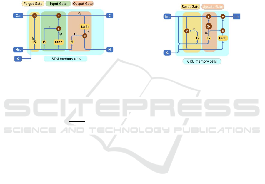
3.3 LSTM
The LSTM modifies the RNN model by designing a
memory cell with selective memory function. It can
memorize valuable information, filter out noise, and
reduce the burden on memory. Figure 2 is a schematic
diagram of the structure of the LSTM model.
Figure 2: LSTM model structure.
𝑐

: The state of memory cells at moment t.
ℎ

: The hidden state at moment t. In many cases, the
hidden state is output directly.
𝑥

: Input data at moment t.
σ: It represents an activation function. In this
experiment it is σ(x)=

(

)
tanh: It represents tanh(x) which can limit the data
to (-1,1).
⊙: It represents the multiplication of two vectors
element by element.
𝑓

: The forget gate at moment t. Decide what
information to forget.
f

=σ(W


x

+W


h

+b

) (4)
𝐼

: Input gate at moment t. Decide which new
memories to generate.
𝑔

: The candidate cell state. New memories are
generated based on the input, but not all of them
are useful and need to be multiplied by 𝐼

.
𝐼

=𝜎(W

x

+W

h

+b

)
(5)
𝑔

=𝑡𝑎𝑛ℎ(W

x

+W

h

+b

)
(6)
𝑂

: Output gate at moment t. Decide what
information to output.
𝑚

: All memories are output according to the state of
the memory cells. After being multiplied with
OT, it can output a useful part.
𝐶

=𝐶

⊙
𝑓

+𝑔

⨀𝐼

(7)
𝑂

=𝜎(W

x

+W

h

+b

)
(8)
𝑚

=𝑡𝑎𝑛ℎ(𝐶

)
(9)
ℎ

=𝑂

⊙𝑚

(10)
3.4 GRU
Compared with LSTM, the GRU model has a simpler
structure. Different from LSTM, an update gate and a
reset gate make up the GRU model. Because it has
fewer parameters, it is not easy to overfit. Figure 3 is
a schematic diagram of the structure of the GRU
model.
Figure 3: GRU model structure.
ℎ

: The hidden state at moment t. In many cases, the
hidden state is output directly.
𝑥

: Input data at moment t.
σ: It represents an activation function. In this
experiment it is σ(x)=

(

)
tanh: It represents tanh(x) which can limit the data
to (-1,1).
⊙: It represents the multiplication of two vectors
element by element.
𝑟

: The reset gate of moment t. It combines the new
input information with previous memories.
𝑟

=𝜎(W

x

+W

h

+b

)
(11)
𝑢

: The update gate of moment t. It removes useless,
repeatable memories and retains useful
memories.
𝑢

=𝜎(W

x

+W

h


+b

)
(12)
ℎ


=𝑡𝑎𝑛ℎ(W


x

+W


(h

⨀r

)
+b


)
(13)
ℎ

=(1−𝑢

)⨀ℎ

+𝑢

⨀ℎ


(14)
4 EXPERIMENT
4.1 Dataset
This experiment uses Netflix (NFLX) stock prices
from 2018.2 to 2022.2 as a data set (Verma, and Arti).
The dataset contains the date, closing price, opening
DAML 2024 - International Conference on Data Analysis and Machine Learning
490

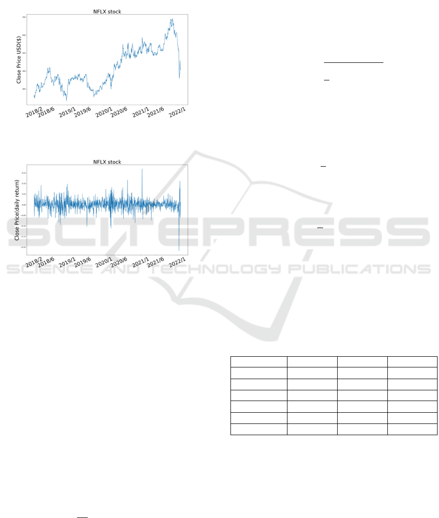
price, volume, and other indicators of the NFLX stock.
In this experiment, the date and closing price are
worth paying attention to. Figure 4 shows the closing
price of NFLX.
Figure 5 shows the daily returns of NFLX .
Figure 4: Closing price of NFLX.
Figure 5: Daily return of NFLX.
In this experiment, 15% of the data was
segmented for detection, and the rest was used for
training.
4.2 Data preprocessing
This experiment uses minmax-scaler as the
normalization method (formula (1))
The control group (CG): directly normalize
the closing price and put it into the RNN, LSTM, and
GRU models as training data.
The experimental group (EG): firstly, convert
the closing price into the form of daily return
(Equation (2))
The second step is to average the daily return in
groups of ten as the data for that day: (𝑑𝑎𝑡𝑎

′ is the
average data of daily return)
data

′=
1
10
dail
y
return



(15)
Then put the average data of daily return into the
RNN, LSTM and GRU models as training data.
4.3 Evaluation metric
In this experiment, RMSE, MAE and MSE were used
as evaluation indicators. In the formula, y represents
the original value, 𝑦 represents the value of
prediction, and n represents how much data there is.
Root Mean Square Error (RMSE) is often used
to evaluate models that predict accurately. Because it
has a square term, it is sensitive to outliers.
RMSE(
y
,
y

)=

1
n
(
y

−
y

)

(16)
Mean Absolute Error (EAS) is a commonly used
loss function that is simple, intuitive, and easy to
calculate. It is suitable for comparison when the error
is obvious, but it is not conducive to the calculation
of gradients。
MAE(
y
,
y

)=
1
n
|
y

−
y

|
(17)
Mean Squared Error (MSE) is a derivable
formula which fit gradient descent algorithm. Also, it
has a square term, so it is sensitive to outliers.
MSE(
y
,
y

)=
1
n
(
y

−
y

)

(18)
4.4 Result
In this experiment, the final data was converted into a
daily return to calculate the RMSE, MAE, MSE.
Table 2 shows a comparison of the prediction
accuracy of the experimental and control groups in
different models.
Table 2: Comparison of CG and EG in different models.
Model RMSE MAE MSE
LSTM(CG) 3.03 × 10

1.82 × 10

9.19 × 10

LSTM(EG) 4.96 × 10

4.96 × 10

2.46 × 10

GRU(CG) 3.17 × 10

1.94 × 10

1.01 × 10

GRU(EG) 3.89 × 10

3.89 × 10

1.51 × 10

RNN(CG) 5.28 × 10

3.65 × 10

2.79 × 10

RNN(EG) 8.99 × 10

7.84 × 10

8.09 × 10

In the experiment, the effects of CG and EG
predictions in different models are also plotted.
Figure 6 is a comparison of stock prices predicted
using LSTM for the experimental and control groups.
Figure 7 is a comparison of stock prices predicted
using GRU for the experimental and control groups.
Figure 8 is a comparison of stock prices predicted
using RNN for the experimental and control groups
Train Recurrent Neural Network to Predict Stock Prices Using Daily Return Rate
491

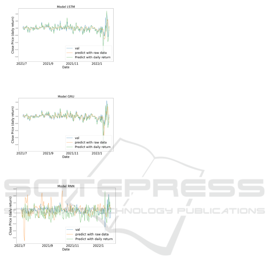
Figure 6: CG and EG predict results in LSTM.
Figure 7: CG and EG predict results in GRU.
Figure 8: CG and EG predict results in RNN.
5 CONCLUSIONS
An in-depth analysis of the experimental data in
Table 2 shows a significant conclusion: the use of
daily returns as an input to the forecasting model
significantly improves the accuracy of forecasting
compared to the traditional method of using closing
prices. This finding was validated in three different
recurrent neural network models: LSTM, GRU, and
RNN. Specifically, the use of daily return showed an
increase in predictive power across all models, but
this improvement was particularly significant in the
GRU model, while the improvement effect was
relatively small in the RNN model.
This difference may be due to the unique
structural characteristics of the GRU model, which
effectively controls the flow of information through
update gates and reset gates, allowing the model to
better capture short-term dynamic changes in time
series data, which is especially important for data
with high frequency changes such as daily returns. In
contrast, RNN models may not be as effective as
GRU and LSTM models in dealing with such
complex data due to their simple structure, especially
in capturing long-term dependencies. Although the
LSTM model also shows a good performance
improvement, it may not have a significant
improvement effect when processing the daily return
data as well as the GRU model due to its more
complex gating mechanism.
These results further confirm the potential of
daily returns as an input to predictive models,
especially when using models such as GRU that can
efficiently handle short-term dynamic changes. This
finding has important practical implications for
financial analysts and investors, as it provides a new
perspective to improve stock market forecasting
models, which may lead to better investment
decisions and risk management strategies.
REFERENCES
Gao, Y., Wang, R., & Zhou, E. (2021). Stock prediction
based on optimized LSTM and GRU
models. Scientific Programming, 2021(1), 4055281.
Ghosh, A., Bose, S., Maji, G., Debnath, N., & Sen, S. (2019,
September). Stock price prediction using LSTM on
Indian share market. In Proceedings of 32nd
international conference on (Vol. 63, pp. 101-110).
Jahan, I., & Sajal, S. (2018). Stock price prediction using
recurrent neural network (RNN) algorithm on time-
series data. In 2018 Midwest instruction and
computing symposium. Duluth, Minnesota, USA:
MSRP.
Lase, S. N., Yenny, Y., Owen, O., Turnip, M., & Indra, E.
(2022). Application of Data Mining To Predicate
Stock Price Using Long Short Term Memory
Method. INFOKUM, 10(02), 1001-1005.
Moghar, A., & Hamiche, M. (2020). Stock market
prediction using LSTM recurrent neural
network. Procedia computer science, 170, 1168-1173.
Patel, J., Patel, M., & Darji, M. (2018). Stock price
prediction using RNN and LSTM. Journal of
Emerging Technologies and Innovative
Research, 5(11), 1069-1079.
Pawar, K., Jalem, R. S., & Tiwari, V. (2019). Stock market
price prediction using LSTM RNN. In Emerging
DAML 2024 - International Conference on Data Analysis and Machine Learning
492

Trends in Expert Applications and Security:
Proceedings of ICETEAS 2018 (pp. 493-503).
Springer Singapore.
Pramod, B. S., & Pm, M. S. (2020). Stock price prediction
using LSTM. Test Engineering and Management, 83,
5246-5251.
Rekha, G., D Sravanthi, B., Ramasubbareddy, S., &
Govinda, K. (2019). Prediction of stock market using
neural network strategies. Journal of Computational
and Theoretical Nanoscience, 16(5-6), 2333-2336.
Selvin, S., Vinayakumar, R., Gopalakrishnan, E. A., Menon,
V. K., & Soman, K. P. (2017, September). Stock price
prediction using LSTM, RNN and CNN-sliding
window model. In 2017 international conference on
advances in computing, communications and
informatics (icacci) (pp. 1643-1647). IEEE.
Singh, R., & Srivastava, S. (2017). Stock prediction using
deep learning. Multimedia Tools and Applications, 76,
18569-18584.
Srivastava, P., & Mishra, P. K. (2021, October). Stock
market prediction using RNN LSTM. In 2021 2nd
Global Conference for Advancement in Technology
(GCAT) (pp. 1-5). IEEE.
Verma, S., & Arti, S. Prediction of Netflix Stock Prices
using Machine Learning. Learning, 1(2), 9-14.
Zhong, X., & Enke, D. (2019). Predicting the daily return
direction of the stock market using hybrid machine
learning algorithms. Financial innovation, 5(1), 1-20.
Zhou, J. (2024). Predicting Stock Price by Using Attention-
Based Hybrid LSTM Model. Asian Journal of Basic
Science & Research, 6(2), 145-158.
Train Recurrent Neural Network to Predict Stock Prices Using Daily Return Rate
493