Comparative Analysis of ARIMA and Deep Learning Models for

Time Series Prediction

Chenyu Jiang

School of Economics and Management, Xidian University, Xi’an, China

Keywords: Time Series Analysis, ARIMA, RNN, LSTM.

Abstract: Time series analysis is crucial for forecasting future trends across various complex real-world domains,

including finance, healthcare, and energy management. This study evaluates the performance of traditional

and deep learning approaches for time series prediction, comparing the autoregressive Integrated Moving

Average (ARIMA) model with Recurrent Neural Network (RNN) and Long Short-Term Memory (LSTM)

architectures. ARIMA, which is designed for linear and stationary data, was tested on the Corona Virus

Disease (COVID)-19 dataset to predict infection rates. While ARIMA achieved reasonable success, its

limitations became apparent in handling non-linear data. Conversely, RNN and LSTM models excelled in

capturing complex non-linear patterns and temporal dependencies, demonstrating superior performance in

forecasting a large-cap stock dataset. The experimental results revealed that LSTM significantly outperformed

ARIMA in prediction accuracy. This underscores the growing need to integrate statistical models like ARIMA

with deep learning techniques to enhance time series forecasting. The findings are particularly relevant for

forecasting applications across industries, suggesting that hybrid models, which balance interpretability with

predictive performance, may offer the most effective solutions.

1 INTRODUCTION

Time series analysis is a basic statistical and

computational process for detecting statistics about

sequences of data points that have been all obtained

in successive details with specific spans. However, it

is very important in many applications such as

finance, meteorology energy management, and

healthcare for a better understanding of hidden

behaviors behind real-world data series that may help

to predict future trends leading to good decision-

making (Torres et al., 2021). Time series analysis is

primarily used to analyze data, identify trends, and

predict future outcomes by considering the

dependencies that exist over time. Time series

theories are natural phenomena from over time, that

help in linear predictions by defining human pattern

characteristics on monthly and seasonal turns through

models like Auto Regressive Moving Average

(ARMA) & Seasonal Auto Regressive Integrated

Moving-Average (SARIMA). Even for simple

scaling, they still face difficulty at times to

accommodate high non-linearities and data that

https://orcid.org/0009-0005-4543-7972

exhibit complex patterns, especially in the presence

of higher dimensions or if the system is not stationary

(Lim and Zohren, 2021).

With growing complexity of data, innovation is

the call-to-action for this new kind of modern time

series data and work. Consequently, numerous

studies are prompting more sophisticated algorithms

to develop where machine learning and deep learning

are combined. Overall, this work has demonstrated an

ability to address the constraints of traditional models

by offering more sophisticated predictive

performance as well as enabling new rules on

architecture and data format. Hence, the study of time

series analysis techniques is indispensable and

important in both research and numerous real-world

applications (Shen et al., 2020).

The area of time series analysis has made very

strong marks recently, notably in the era when

machine learning and deep-learning techniques rule.

Among the traditional methods, ARMA and

SARIMA are still widely used for their simplicity to

implement quickly, yet they perform well on some

time series datasets. They are well-suited for linear,

306

Jiang and C.

Comparative Analysis of ARIMA and Deep Learning Models for Time Series Prediction.

DOI: 10.5220/0013516200004619

In Proceedings of the 2nd International Conference on Data Analysis and Machine Learning (DAML 2024), pages 306-310

ISBN: 978-989-758-754-2

stationary data and renowned for their interpretability

(Sezer et al., 2020). However, the efficiency of

Recurrent Neural Networks (RNNs) declines in

tackling nonlinearity, long-term dependencies as well

as high-dimensional data.

In response to these challenges, researchers are

more frequently using deep learning models such as

RNNs and Long Short-Term Memory (LSTM)

networks. Since sequence data can be serialized in

time, RNN comes up with stronger performance at

modeling temporal patterns. LSTM networks are one

type of RNN more designed for long-term

dependency communication and bypass the standard

neural network training issue caused by gradient

decay (Zeng et al., 2023). These models have

demonstrated state-of-the-art performance in various

applications, including stock market prediction,

weather forecasting, and natural language processing,

by effectively capturing the complex, non-linear

relationships present in data. More recently, it has

been seeing a rise in interest starting to use new

methods such as Graph Neural Networks (GNNs) and

Transformer models for time series analysis (Satrio et

al., 2021). GNNs are especially useful for encoding

features of nodes in the graph since they model node

dependencies (social networks or financial

interconnected systems) through structural properties

(Mao and Xiao, 2019). Transformer models, designed

for originally the Natural Language Processing (NLP)

domain have also shown great promise in time series

forecasting modeling large datasets efficiently, and

capturing long-range dependencies (Zeng et al.,

2023). Insight into what these cutting-edge models

mean for time series analysis and how new

advancements can be used to predict more accurately,

as well as glean actionable insights from the data.

This study aims to systematically review

foundational technologies for analyzing time series

data, addressing a gap in comparative analysis and

methodological connections. The paper provides a

thorough review of evolving paradigms in time series

analysis, outlining major philosophies and distilling

key concepts to assist beginners re-entering the field.

It also offers insightful perspectives on

methodologies designed to handle increasingly

complex high-dimensional non-linear data. The study

highlights successful applications of these

technologies through real-life case studies, detailing

their benefits and limitations. Additionally, it

provides a brief overview of future trends and

potential research directions. By synthesizing current

methodologies and exploring practical applications,

this paper aims to enhance understanding and guide

future investigations in time series analysis.

2 METHODOLOGY

2.1 Data Modeling and Analysis

Principles

This research applies two primary methods for time

series prediction: the classical ARIMA model and

modern deep learning techniques such as RNNs and

LSTMs. ARIMA model, useful for linear and

stationary data, uses auto regression, differencing,

and moving average techniques for forecasting.

Meanwhile, its major advantage of being easily

interpretable, the application of ARIMA for analysis

of non-linear and non-stationary data reduces its

efficiency. On the other hand, RNNs especially

LSTMs-are categories of neural networks introduced

to model and depict non-linear processes in the

temporal data. Such structures as memory cells make

LSTMs ideal for temporal forecasting due to the

ability to capture long-term dependencies. This work

discusses the performance of both ARIMA and

LSTM models when applied to different datasets and

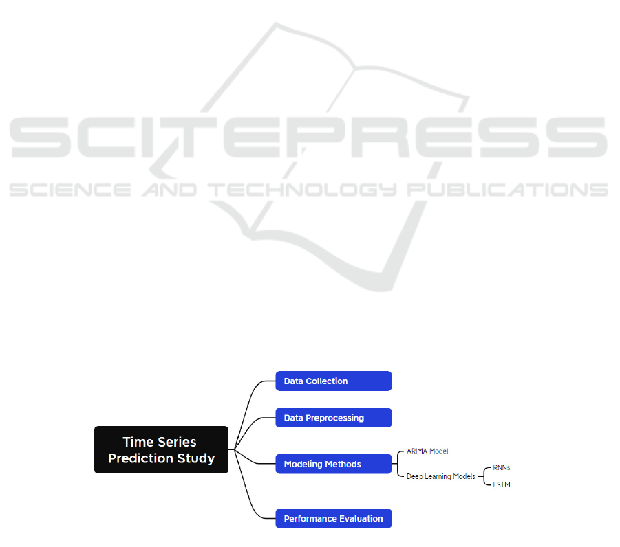
different situations. A described flowchart of the

methodology pipeline for this research is provided in

Figure 1 below.

Figure 1: The time series prediction study pipeline (Picture credit: Original).

Comparative Analysis of ARIMA and Deep Learning Models for Time Series Prediction

307

2.2 ARIMA Model

2.2.1 Dataset Description

The ARIMA model was applied to a dataset tracking

the spread of the Corona Virus Disease (COVID-19)

epidemic, sourced from Johns Hopkins

epidemiological records. This dataset includes time-

stamped information on infection rates, recoveries,

and other pandemic-related statistics. It is particularly

suited for ARIMA, which requires stationary time

series data for effective prediction. The goal is to

predict the incidence and prevalence of COVID-19

over time, leveraging ARIMA’s ability to model and

forecast linear trends in the data. This dataset is

described in the study Application of the ARIMA

model on the COVID-2019 epidemic dataset

(Benvenuto et al., 2020).

2.2.2 Core Technology

The ARIMA is a common statistical model in

analyzing time series data especially when the series

is linear and stationary. It integrates three

components. First, Auto-Regressive (AR)

Component – this part describes the connection

between an observation and certain previous

observations (or earlier time points). Next, the

Integrated (I) Component is the differencing of raw

observations to render the time series stationary. This

step helps in the removal of trends which helps in

making the model trendless by focusing on variations

around the mean. Lastly, the Moving Average (MA)

Component, this part captures the dependence of an

observation on the residual errors from a moving

average model of lagged observations.

For this application, ARIMA requires the tuning

of three parameters: p stands for the order of the AR

term, d for the degree of differencing, and q for the

order of the MA term. These parameters are normally

selected from statistics on model performance on the

validation data using statistics such as the Akaike

Information Criterion (AIC). Even though the

ARIMA model is quite easy to apply, there are

restrictions as it cannot handle non-linearity which is

often found in the real time data sets and especially

when exposed to shocks like the COVID-19

Pandemic (Benvenuto et al., 2020).

2.3 RNN and LSTM Models

2.3.1 Dataset Used

For the RNN and LSTM models, a stock market

dataset was utilized, which captures historical stock

prices over time. This dataset is highly volatile, with

stock prices influenced by a variety of external

factors, making it ideal for testing the ability of deep

learning models to capture complex, non-linear

dependencies. The dataset includes time-stamped

records of stock price movements, which allow the

models to learn temporal patterns and make future

price predictions. This dataset is explored in detail in

Predictive Data Analysis: Leveraging RNN and

LSTM Techniques for Time Series Dataset (Agarwal

et al., 2024).

2.3.2 Core Technology

RNNs are special types of neural networks that are

used to work with sequences of data. Neural networks

work beyond others in series where inputs are

processed independently from each other whereas

RNNs take feedback of the output and pump back into

the network. This looping mechanism empowers

RNNs to grasp temporal dependencies. Nonetheless,

RNNs face serious challenges, notably the vanishing

gradient problem where gradients reduce as they are

back-propagated through time making it hard for the

model to learn long term dependencies.

Therefore, to solve the vanishing gradient issue,

an LSTMs architecture is recommended. To

overcome this challenge, LSTMs have a memory cell

reserved for the whole sequence. This is by an input

gate which determines what information with regard

to the inputs should be used in updating memory.

Another known type is the forget gate which

determines which parts of the cell states it needs to

remember or forget and the output gate or the pseudo-

gate which has a similar function to patterns of what

it wants to reveal along with the final results. This

enclosed structure allows LSTM to maintain the

information that is important, and discard the rest, for

long periods, and is ideal for assessing future values

from a long range of previous and current values. In

the stock market application, LSTMs perform much

better than traditional RNNs and other models since

LSTMs address the vanishing gradient problem

inherent in highly volatile time series data while

incorporating the long-term dependencies. In one

application, LSTM was found to predict with an

accuracy of 91.97% was achieved on testing data

(Agarwal et al., 2024).

DAML 2024 - International Conference on Data Analysis and Machine Learning

308

The integration of these two models means that

researchers can take the best of conventional

statistical methods and modern deep learning and

apply them to improved time series prediction in

various situations.

3 RESULT AND DISCUSSION

3.1 The Performance of Models

As indicated in Table 1, the two techniques; ARIMA

and RNN/LSTM provide somewhat different results

in terms of time series prediction. The accuracy of the

ARIMA model was high not only in the case of short

periods of observations but also in cases of relatively

simple and linear data, such as the dynamics of

COVID cases. But when having to deal with more

complex and non-stationary data like the stock market

data, the accuracy of the ARIMA method is reduced.

When the nature of the data was more volatile and

complex, the errors made in prediction also tended to

rise. Conversely, based on the nature of the RNN-

LSTM model, which was created to handle non-linear

and more complex trends, the model yielded

significantly more accurate long-term predictions,

especially, if the data set was intrinsically volatile.

Among them, the LSTM model had better results by

learning long-term dependencies and trends in stock

market data and outperformed the overall

performance of ARIMA.

Table 1: Different results in terms of time series prediction.

Feature ARIMA Model RNN/LSTM

Models

Data Type Linear,

stationary data

Non-linear,

complex data

Model

Characteristics

Simple, easy to

understan

Complex, harder

to understan

Prediction

Abilit

Good for short-

term

redictions

Good for long-

term

redictions

Data Needs Small datasets Requires a lot of

data

Computational

Power

Low

computational

needs

High

computational

needs

Performance Good for simple

data

Better for

complex,

volatile data

Training Time Quick to train Takes longer to

train

Best Use Simple

forecasting

tasks

Complex

forecasting tasks

Limitations Struggles with

complex data

Can overfit,

requires more

resources

3.2 Discussion

The study reveals the strengths and limitations of

using the ARIMA and the neural network models.

ARIMA is recommended for tasks where high

interpretability is important, and where the data is

linear and stationary since it can be deployed quickly

and implemented with low computational power.

However, it falters when it comes to non-linear data

and conditions that are characterized by sudden

changes in trends. However, when it comes to non-

linear and non-stationary datasets, the performance of

the RNN and LSTM models are found to be

significantly better due to their capability of learning

from the long-term dependency. Although, these

models offer better data estimations especially on the

volatile data such as stock prices, they possess higher

computational complexities and need large data sets

for training. However, training these neural networks

takes time; therefore, they are not very suitable for

projects that have limited data or computing power.

Future work can explore the integration of the

ease of use of ARIMA model with the powerful

forecasting performance of RNN and LSTM. Such a

combination might prove a more effective

compromise between the interpretability of ARIMA

and the higher accuracy of neural networks. However,

if training becomes less time-consuming and requires

fewer data for deep learning models, it expands their

application and usability in forecasting.

4 CONCLUSIONS

The results presented here prove some advantages

and drawbacks of the ARIMA models and the neural

network-based solutions. ARIMA is relatively simple

to implement and maintain given its high

interpretability; it is better suited for linear and

stationary data and provides a fast solution that does

not consume considerable computational power.

Nevertheless, they do not effectively handle non-

linear data and sharp changes of trends, which gives

them less potential in complex forecast assignments.

However, RNN and LSTM models perform very well

with quantitative data sets that display non-linear

features, including cryptocurrency data that are more

inclined to specific time sequences. These models are

very proficient in capturing long term trends and tend

to exhibit higher accuracy for highly oscillatory data,

Comparative Analysis of ARIMA and Deep Learning Models for Time Series Prediction

309

such as stock price data. However, RNNs and LSTMs

have significant computational needs and an

extensive amount of training data which can be an

issue for a small-scale project or when a large amount

of data is unavailable. Another potential area for

further research might lie in combining ARIMA with

the advantages of RNNs or LSTMs while keeping

ARIMA’s interpretability in mind. This may provide

a balanced solution by refining the ARIMA’s

forecasting capability and at the same time keeping it

simple. Moreover, improvements in the training itself

as well as handling of the data could bring the deep

learning models to a wider range of applications for

forecasting.

REFERENCES

Agarwal, H., Mahajan, G., Shrotriya, A., et al. 2024.

Predictive Data Analysis: Leveraging RNN and LSTM

Techniques for Time Series Dataset. Procedia

Computer Science, 235, 979-989.

Benvenuto, D., Giovanetti, M., Vassallo, L., et al. 2020.

Application of the ARIMA model on the COVID-2019

epidemic dataset. Data in brief, 29, 105340.

Lim, B., Zohren, S., 2021. Time-series forecasting with

deep learning: a survey. Philosophical Transactions of

the Royal Society A, 379(2194), 20200209.

Mao, S., Xiao, F., 2019. Time series forecasting based on

complex network analysis. IEEE Access, 7, 40220-

40229.

Satrio, C.B.A., Darmawan, W., Nadia, B.U., et al. 2021.

Time series analysis and forecasting of coronavirus

disease in Indonesia using ARIMA model and

PROPHET. Procedia Computer Science, 179, 524-532.

Sezer, O.B., Gudelek, M.U., Ozbayoglu, A.M., 2020.

Financial time series forecasting with deep learning: A

systematic literature review: 2005–2019. Applied soft

computing, 90, 106181.

Shen, Z., Zhang, Y., Lu, J., et al. 2020. A novel time series

forecasting model with deep learning.

Neurocomputing, 396, 302-313.

Torres, J.F., Hadjout, D., Sebaa, A., et al. 2021. Deep

learning for time series forecasting: a survey. Big Data,

9(1), 3-21.

Zeng, A., Chen, M., Zhang, L., et al. 2023. Are transformers

effective for time series forecasting? Proceedings of the

AAAI conference on artificial intelligence. 37(9),

11121-11128.

DAML 2024 - International Conference on Data Analysis and Machine Learning

310