Traffic Prediction Using LSTM, RF and XGBoost

Ka Nam Lam

School of Mathematics, University of Bristol, Fujian, China

Keywords: Traffic Flow Prediction, Machine Learning, LSTM, XGBoost, Random Forest.

Abstract: Traffic congestion is one of the most challenging and lasting problems that causes many government concerns.

It would lead to many problems, such as economic losses, fuel consumption, environmental costs, and so on.

An efficient traffic system can significantly reduce congestion, which can bring many beneficial impacts on

daily life. Accurate traffic flow prediction is crucial for effective traffic management. This study uses three

machine learning models: Random Forest (RF), Extreme Gradient Boosting (XGBoost), and Long Short-

Term Memory (LSTM) to predict vehicle counts at four different junctions of a city. Each of these models

was evaluated based on key metrics – Mean Absolute Error (MAE), Root Mean Squared Error (RMSE), and

R-squared (𝑅



). The outcomes showed that XGBoost performed the best among the examined models in

terms of precision and computational efficiency. This paper also discusses the limitations of the models and

future implications, which can be helpful in better managing transportation systems.

1 INTRODUCTION

Traffic congestion is a chronic problem affecting

urban environments globally, which may be caused

by high population density, increased number of

vehicles, and infrastructural development (Vencataya

et al., 2018). Therefore, effectively managing the

traffic system is one of the most significant issues

faced by modern cities nowadays. Accurate traffic

flow prediction is an essential component of an

intelligent traffic system. However, predicting traffic

is very complex due to its dynamic nature, as

researchers must consider various factors, including

peak hours, weather conditions and special events.

These factors are not correlated linearly, so traffic

prediction becomes a challenging problem that

requires more advanced analytical methods/models

(Hong et al., 2015; Joaquim et al., 2015).

Over the years, many methods have been used to

address the traffic prediction issue. In the last decade,

researchers have commonly used statistical

approaches, such as Autoregressive Integrated

Moving Average (ARIMA) and Kalman filters,

which have been the most studied techniques for time

series forecasting. These methods are well-suited for

simple linear relationship problems. However, traffic

prediction is a complex spatial problem. Thus, they

https://orcid.org/0009-0003-9338-1956

presented difficulties in addressing such predictions

(Medina-Salgado et al., 2022). Researchers have

developed new methods to better manage traffic

predictions and deal with new challenges.

Several machine learning techniques have been

developed for traffic prediction. For example, models

like Support Vector Machine (SVM), K-nearest

Neighbors (KNN) and Artificial Neural Networks

(ANN) have achieved better results to a certain

degree, as they can better capture the non-linear

patterns in the traffic data, thus becoming more

appropriate choices for this problem. For example,

Hong et al. (2015) proposed a hybrid multi-metric

KNN model for the forecast of traffic flow, which

showed better accuracy in combining a set of metrics

to capture different data patterns.

Furthermore, many researchers have also used

tree-based machine learning models such as Random

Forest (RF) and Extreme Gradient Boosting

(XGBoost) because they can bear more complex data

entries. For instance, Wang and Fang (2024)

combined XGBoost with wavelet analysis to improve

short-term traffic flow prediction. They demonstrated

the model’s efficiency and precision in capturing

periodic patterns.

Deep learning models, especially Long Short-

Term Memory (LSTM) networks, have recently been

Lam and K. N.

Trafﬁc Prediction Using LSTM, RF and XGBoost.

DOI: 10.5220/0013515600004619

In Proceedings of the 2nd International Conference on Data Analysis and Machine Learning (DAML 2024), pages 267-274

ISBN: 978-989-758-754-2

267

trending in traffic prediction. As LSTM networks are

designed to process sequential data and are capable of

memorizing information for a long period of time, so

this model is suitable for operating on time series

data. LSTM models have been widely applied in

various studies, especially in time series data

forecasting, and their good performance has been

proven accordingly. For instance, Ye et al. (2024)

carried out a thorough analysis of traffic flow

prediction by LSTM networks and outlined the

capability for modelling complicated temporal

dependencies in traffic data. While LSTM has many

merits, its drawbacks might be long computational

time and large sizes of datasets to achieve optimal

performance.

The main objective of this study is to identify a

machine learning model that can accurately predict

traffic flow at different junctions of a city. This study

considers three kinds of machine learning models:

LSTM Networks, RF, and XGBoost. These models

have unique advantages regarding handling time

series data, non-linear relationships, and feature

importance, making them suitable for traffic

prediction. The study evaluates the performance of

these models by metrics such as Mean Absolute Error

(MAE), Root Mean Squared Error (RMSE) and R-

squared (𝑅



) to determine the most effective model

for traffic prediction.

The rest of the article is structured as follows:

Section 2 discusses the methodology used in this

paper, involves data preprocessing steps, model

description, and the metric used to evaluate models’

performance. Section 3 presents the results of the

model evaluations and compares their performances

based on key metrics. Section 4 discusses the

limitations of the study and the future works that

could improve the models. Finally, the conclusions

are drawn in Section 5.

2 DATA PREPARATION AND

MODEL OVERVIEW

2.1 Dataset Overview

Table 1: Dataset sample.

Date Time Junction Vehicles ID

2015-11-01

00:00:00

1 15 20151101001

2015-11-01

01:00:00

1 13 20151101011

2015-11-01

02:00:00

1 10 20151101021

2015-11-01

03:00:00

1 7 20151101031

The dataset used in this project was sourced from

Kaggle (Fedesoriano, 2021). It contains vehicle

counts across four junctions over several years. The

dataset contains 48120 rows of data, with each row

representing an individual traffic observation. Each

observation has features shown in Table 1, including

DateTime: the exact time of the observation, which

indicates the month, day, and hour; Junction: the

junction number where the observation was recorded;

Vehicles: the number of vehicles passing through the

junction at the time; Unique ID: an identifier for the

row data. The target variable was the number of

vehicles for the next hour.

2.2 Data Preprocessing

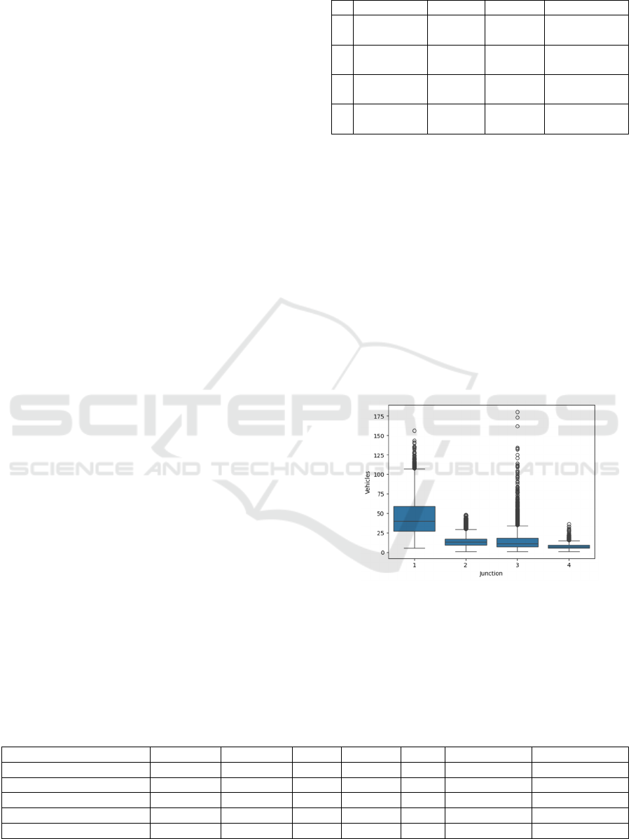
Figure 1: Outliers of vehicle counts for each junction

(Photo/Picture credit: Original).

Data preprocessing is a critical step in machine

learning model development, particularly for time

series data such as traffic data, to enable models to

learn

and analyze the patterns in data effectively.

Table 2: Dataset after feature engineering.

DateTime Junction Vehicles Yea

Month Da

Hou

of wee

2015-11-01 00:00:00 1 15 2015 11 1 0 6

2015-11-01 01:00:00 1 13 2015 11 1 1 6

2015-11-01 02:00:00 1 10 2015 11 1 2 6

2015-11-01 03:00:00 1 7 2015 11 1 3 6

2015-11-01 04:00:00 1 9 2015 11 1 4 6

DAML 2024 - International Conference on Data Analysis and Machine Learning

268

Table 3: ADF test for vehicle count data.

ADF statistic

-value 1% critical value 5% critical value 10% critical value Stationarit

Junction 1 -7.366837 9.189060e-11 -3.430804 -2.861741 -2.566877 True

Junction 2 -9.151651 2.676498e-15 -3.430830 -2.861752 -2.566883 True

Junction 3 -6.614107 6.269937e-09 -3.430815 -2.861745 -2.566879 True

Junction 4 -6.378744 2.249640e-08 -3.431901 -2.862225 -2.567135 True

First, feature engineering was conducted. Temporal

features such as year, month, day, hour, and day of

the week were created to capture cyclical patterns in

traffic, as shown in Table 2. Additionally, for

preparing the data with the LSTM model, a sliding

window approach was used to create sequences of

historical data. This approach allows the model to

capture more local patterns and learn efficiently.

Second, data cleaning was performed by detecting

and eliminating outlier data in the dataset to prevent

the models from misinterpreting the dataset due to

anomalous data points. Figure 1 depicts the detected

outliers, which do not represent normal road

conditions due to special events like accidents or road

closures, as the number of vehicles at the specific

time was typically large, showing congestion. When

these anomalies are eliminated, the data can represent

typical traffic patterns.

After the creation of temporal features, the

normalisation was performed to scale vehicle counts.

This would keep all data ranges consistent for better

and more stable model performance. Lastly, as seen

in Table 3, the Augmented Dickey-Fuller (ADF) test

was conducted to check for stationary in the vehicle

count data. The stationarity of data is critical for time

series models. It ensures that the data’s statistical

properties, such as the mean and variance, do not

change over time. If the stationary test showed that

the data were stationary (ADF test result is True),

then the data could be used for further modelling

directly. However, if the data were non-stationary

(ADF test result is False), differencing needs to be

applied on the data to remove any trends, making the

data stationary.

2.3 Models

This paper uses the following models to predict traffic

flow: RF, XGBoost, and LSTM.

RF is an ensemble learning method that builds

many decision trees and merges their results to make

predictions. This model is robust to overfitting and

can demonstrate the importance of different features

(Akhtar & Moridpour, 2021), which is vital for

understanding the contribution of different features in

the prediction.

XGBoost is an advanced tree-based gradient

boosting algorithm, which is well-known for its high

efficiency. It can handle complex interactions in

structured data and process data features in parallel.

Additionally, XGBoost has been known for its high

precision and accuracy. Supported by a gradient

boosting framework, the model reduces the error by

minimizing a loss function, such as MSE. This

iterative approach improves the model’s precision at

each iteration step, therefore, presents an enhanced

prediction ability of the model (Dong et al., 2018;

Wang & Fang, 2024). Thus, high computational

efficiency and precision make XGBoost a strong

choice for traffic flow prediction.

LSTM is a recurrent neural network (RNN) class

that works particularly well in time series prediction

applications. LSTM is able to capture long-term

dependencies and temporal features in time series

data, which are crucial for the accurate prediction of

traffic patterns in time series. Unlike typical RNN

networks that may struggle with the problem of

vanishing gradients, the LTSM can keep information

over more extended periods thanks to the internal

gating mechanisms. In addition, LSTM can learn the

data patterns itself without extra feature engineering,

which is often required for many machine learning

models (Ye et al., 2024). Therefore, these properties

of LSTM make it a powerful model for traffic

forecasting.

3 EXPERIMENT RESULTS

Cross-validation and hyperparameter tuning

techniques were applied prior to the performance

evaluation of the model. Firstly, cross-validation test

was performed to assess the models’ performance on

various sets of data to ensure their robustness.

Further, hyperparameter tuning was also conducted

by using the Python built-in function GridSearchCV

to fine-tune the hyperparameters of models for the

best model predictive accuracy.

Trafﬁc Prediction Using LSTM, RF and XGBoost

269

3.1 Experiment Evaluation

It is necessary to establish some metrics in order to

evaluate the performance of the models. For instance,

RMSE, MAE, and R

may be chosen. RMSE could

present a general indicator, which is computed as the

root of the average squared difference between

predictions and actual values (Joaquim et al., 2015).

MAE is a metric used to calculate the average

absolute error/difference between predicted values

and actual values. This value is less sensitive to large

errors than the RMSE value (Joaquim et al., 2015). R

is a statistical measure that shows how well models

explain variance in the target variable (Jiang, 2022).

Collectively, these metrics offer a complete

understanding of the models in the prediction of

traffic patterns.

3.2 Results of Random Forest

Table 4: Performance Metrics of the Random Forest model.

RMSE MAE

𝑅



Junction 1 0.185797 0.136094 0.968583

Junction 2 0.099772 0.080631 0.854158

Junction 3 0.152084 0.114155 0.806105

Junction 4 0.096277 0.077159 0.550362

Table 4 shows the experiment result of the Random

Forest model at four different junctions. Junction 4

owns the smallest RMSE and MAE values, meaning

that the RF model had the most accurate prediction at

this junction. The highest 𝑅



value was achieved at

Junction 1, meaning that the model was able to

explain approximately 96.9% of the variance in the

target variable. Junction 4 has the lowest value of

0.55, so the model was struggling to capture the

variance.

(a) (b)

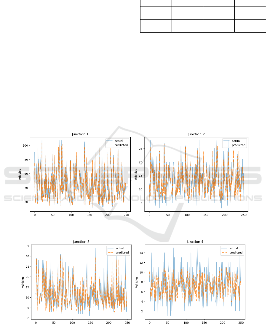
Figure 2: Actual vs. predicted values using Random Forest for 4 junctions. (a): Junction 1, (b): Junction 2, (c): Junction 3,

(d): Junction 4. (Photo/Picture credit: Original).

DAML 2024 - International Conference on Data Analysis and Machine Learning

270

The visualizations demonstrate the numerical

results in Figure 2. As suggested in Figure 2, Junction

1 had the largest RMSE, so plot (a) has more

unmatched patterns, and it captured the variance well.

This aligns with the high 𝑅



value observed in the

metrics table. Also, almost all predictions in the

Junction 4 plot closely fall in the actual value line, so

the RMSE for this junction is the lowest. However,

the model had more difficulty capturing traffic

patterns as the plot demonstrates an obvious

difference in the variances. The table and plots clearly

highlight where the model performed well while still

needing improvement. Junctions 1 and 2 were

accurately predicted, showing the model’s solid

predictive performance. However, the big difference

in variances for junction 4 suggests that the model

could be improved through further tuning or

additional feature engineering.

3.3 Results of XGBoost

Table 5: Performance of XGBoost model.

RMSE MAE

𝑹

𝟐

Junction 1 0.160097 0.118387 0.976673

Junction 2 0.096931 0.078455 0.862345

Junction 3 0.148890 0.111268 0.814165

Junction 4 0.097115 0.077715 0.542502

Table 5 shows that the model performed well at

junctions 1 and 2, with high 𝑅



values and low errors.

Similar to the RF model, the XGBoost model

struggled with junction 4, with the lowest 𝑅



value of

0.54. This means that it was also difficult to capture

the traffic patterns for the XGBoost model.

(a) (b)

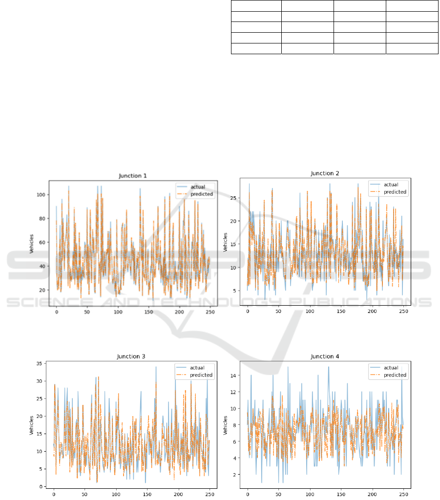
Figure 3: Actual vs. predicted values using XGBoost for 4 junctions. (a): Junction 1, (b): Junction 2, (c): Junction 3, (d):

Junction 4. (Photo/Picture credit: Original).

Trafﬁc Prediction Using LSTM, RF and XGBoost

271

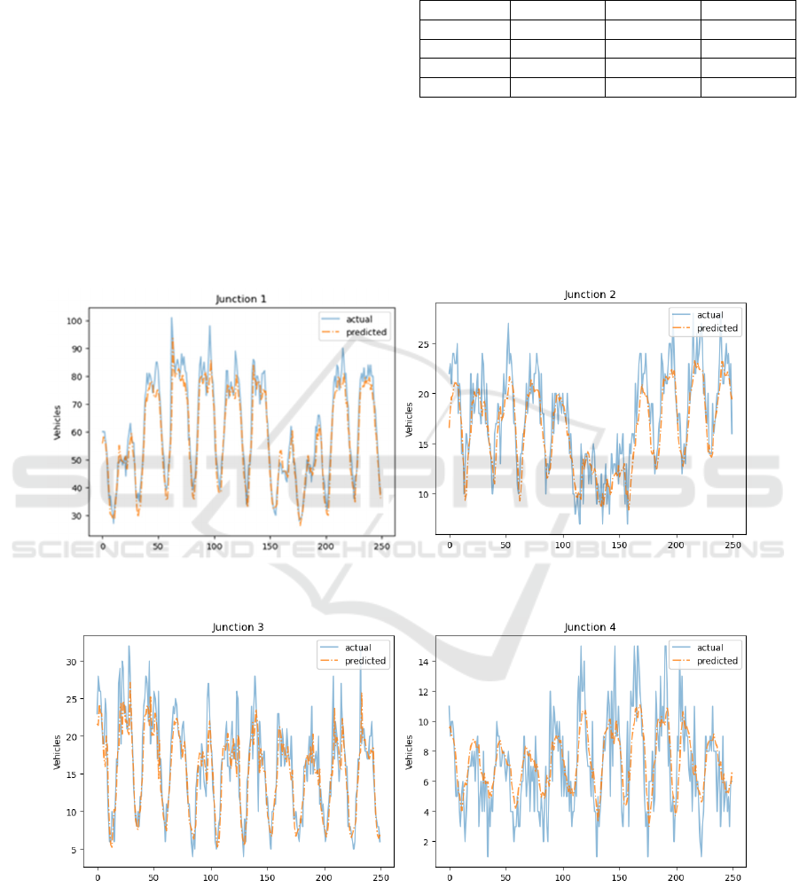
Figure 3 illustrates that the model functioned well

at 1 and 2 junctions, as the predicted vehicle counts

aligned well with the actual values. Junction 3 had

slightly more deviations, suggesting a lower 𝑅



value. The fourth junction showed an even more

significant deviation, indicating that the model did

not interpret the traffic forecasts well. Like the

Random Forest model, this model also needs more

analysis and adjustments to reduce the deviation for

junction 4 and to enhance the overall performance.

3.4 Results of LSTM

Table 6: Performance of LSTM model.

RMSE MAE

𝑅



Junction 1 0.410605 0.320683 0.842318

Junction 2 0.176028 0.143766 0.453334

Junction 3 0.171220 0.131704 0.767415

Junction 4 0.116788 0.091637 0.425882

As shown in Table 6, junction 1 had large prediction

errors compared to the other two models and a

relatively high 𝑅



value. Junctions 2 and 4 both have

a meagre 𝑅



value, suggesting the model did not fit

well with the traffic data. For junction 3, the model

performed relatively well with a moderate 𝑅



value

of 0.77 and relatively low RMSE and MAE.

(a) (b)

Figure 4: Actual vs. predicted values using LSTM for 4 junctions. (a): Junction 1, (b): Junction 2, (c): Junction 3, (d): Junction

4. (Photo/Picture credit: Original).

DAML 2024 - International Conference on Data Analysis and Machine Learning

272

The first and third plots in Figure 4 show that the

predictions of these two junctions generally follow

the trend of the actual values with an apparent

deviation. The model had difficulty capturing the

patterns at both junctions 2, 4, as great deviations

were illustrated in the plots. The model was able to

capture some temporal dependencies, but it is clearly

not as competitive as the others, which may be due to

the lack of data and information.

3.5 Model Comparison

Table 7: The average results of experiment models.

RMSE MAE

𝑅



RF 0.133482 0.102010 0.794802

XGBoost 0.125758 0.096456 0.798921

LSTM 0.218660 0.171947 0.622237

It can be noticed from Table 7 that XGBoost

outperformed both LSTM and RF in terms of all three

metrics. It had the lowest errors on average across all

junctions - RMSE of 0.125758 and MAE of

0.096456. Also, it yielded the highest 𝑅



value of

0.798921, slightly higher compared to the Random

Forest model. Therefore, from these results, it appears

that the XGBoost model can accurately predict and

explain the variance in traffic data across various

junctions.

The RF model also performed very well, with

slightly lower values in all the key metrics. It

achieved an average RMSE of 0.133482, MAE of

0.096456 and 𝑅



of 0.794802. Additionally, the

model could provide the interpretation of the

importance of features, which is also an important

indicator for model development. Thus, this model is

also a powerful model for traffic prediction.

Although LSTM is a robust neural network that is

particularly suitable for time series prediction, it did

not perform as well as the other two models. The

LSTM had the lowest 𝑅



value of 0.622237, the

highest RMSE of 0.21866 and MAE of 0.171947. In

this context of traffic prediction, LSTM was less

accurate in predicting traffic counts, especially in

junctions 2 and 4, with shallow 𝑅



values. Therefore,

the model probably requires further tuning or

additional features and information to compete with

XGBoost and RF.

In summary, XGBoost is the best-performing

model overall. It has the most accurate prediction

results and can capture the variance in the traffic data.

These properties make this model the most reliable

and suitable choice for traffic prediction in this study.

4 LIMITATIONS

This study demonstrated the use of machine learning

models like XGBoost in predicting traffic. However,

there are some limitations during the project that

should be noted. First, there is a lack of information

in the dataset used. The dataset only contained a few

features: the datetime and target variable – vehicle

count across various junctions, while more factors

should be considered, such as weather conditions,

road closures, public events, holiday. These might be

the reasons that affect the models to explain variance

in traffic data fully. Therefore, expanding the dataset

and merging additional features could enhance the

models’ performance.

Another limitation is the performance shown by

the LSTM model, which is a preferred choice when

dealing with time series data. LSTM performed

poorly in this context, which may be attributed to

insufficient tuning or data analysis and preprocessing

specific to the needs of LSTM.

Additionally, the models were trained on data

collected from a specific city. The generalizability of

the findings to other cities, locations with different

traffic patterns, and population numbers was not

tested. Thus, including other locations in the dataset

could help the models understand traffic data more

comprehensively.

Lastly, many Machine Learning models, such as

XGBoost, are black-box models, which are inherently

complex, so making it difficult to interpret the results

and understand how the models obtain the

predictions. This “black-box” nature can be a

significant defect, especially in real-time traffic

management systems, where interpretability is

crucial. Adopting methods like SHAP (Shapley

Additive exPlanations) values could help to address

this issue, as they can provide a comprehensive

understanding of feature importance, thus

determining which factors contribute the most to the

model’s decision-making process.

5 CONCLUSIONS

This paper primarily explored and analyzed the uses

of machine learning models – LSTM, RF, and

XGBoost in the prediction of traffic patterns at

different junctions in a city. The results showed that

XGBoost is the most effective and suitable model for

this context since it held the minimum prediction

errors and the maximum 𝑅



values among all the

models studied. RF also excelled in this task, with

Trafﬁc Prediction Using LSTM, RF and XGBoost

273

slightly lower values in the key metrics than

XGBoost. At the same time, the LSTM model,

despite its theoretical strength in handling time series

data, was not as competitive as the other models.

Hence, the LSTM model requires further tuning or

other features to enhance its performance. These

models’ ability to capture traffic patterns makes them

feasible choices for real-time traffic management.

The XGBoost model can achieve more accurate

short-term forecasts, which will manage the traffic

flow, help reduce traffic congestion and enhance

public safety. However, several limitations were also

identified within this study, such as insufficient

features and geographical limitations. Future research

could also involve fine-tuning the LSTM for

improved performance and training models on larger

datasets with a wider variety of features and regions.

By tackling these problems, it would be feasible to

create more reliable and broadly applicable models,

which would offer additional insights into creating a

more effective transportation system.

REFERENCES

Akhtar, M., Moridpour, S., 2021. A Review of Traffic

Congestion Prediction Using Artificial Intelligence.

Journal of Advanced Transportation, 2021, e8878011.

https://doi.org/10.1155/2021/8878011.

Dong, X., Lei, T., Jin, S., Hou, Z., 2018. Short-Term Traffic

Flow Prediction Based on XGBoost. 2018 IEEE 7th

Data Driven Control and Learning Systems Conference

(DDCLS). https://doi.org/10.1109/ddcls.2018.8516114

Fedesoriano., 2021. Traffic Prediction Dataset. Www.

kaggle.com. https://www.kaggle.com/datasets/

fedesoriano/traffic-prediction-dataset.

Hong, H., Huang, W., Xing, X., Zhou, X., Lu, H., Bian, K.,

Xie, K., 2015. Hybrid Multi-metric K-Nearest

Neighbor Regression for Traffic Flow Prediction.

https://doi.org/10.1109/itsc.2015.365.

Jiang, W., 2022. Cellular traffic prediction with machine

learning: A survey. ScienceDirect, 201.

Joaquim, B., Araujo, M., Rossetti, F., 2015. Short-term

real-time traffic prediction methods: a survey.

Portuguese National Funding Agency for Science,

Research and Technology (RCAAP Project by FCT).

https://doi.org/10.1109/mtits.2015.7223248.

Medina-Salgado, B., Sánchez-DelaCruz, E., Pozos-Parra,

P., Sierra, J. E., 2022. Urban traffic flow prediction

techniques: a review. Sustainable Computing:

Informatics and Systems, 35, 100739.

https://doi.org/10. 1016/j.suscom.2022.100739.

Vencataya, L., Pudaruth, S., Dirpal, G., Narain, V., 2018.

Assessing the Causes & Impacts of Traffic Congestion

on the Society, Economy and Individual: A Case of

Mauritius as an Emerging Economy. Studies in

Business and Economics, 13(3), 230–242. https://doi.

org /10.2478/sbe-2018-0045.

Wang, X., Fang, F., 2024. Short-Term Traffic Flow

Prediction Based on Wavelet Analysis and XGBoost.

International Journal of Transportation Engineering and

Technology, 10(1), 15–24. https://doi.org/10.11648/

j.ijtet.20241001.12.

Ye, B.-L., Zhang, M., Li, L., Liu, C., Wu, W., 2024. A

Survey of Traffic Flow Prediction Methods Based on

Long Short-Term Memory Networks. IEEE Intelligent

Transportation Systems Magazine, 2–27.

https://doi.org/ 10.1109/mits.2024.3400679.

DAML 2024 - International Conference on Data Analysis and Machine Learning

274