Using Neural Networks to Build an Efficient Classification Model for

Classifying Images in the CIFAR-10 Dataset

Yu Huang

Shenzhen College of International Education, Shenzhen, Guangdong, 518043, China

Keywords: Deep Learning, Machine Learning, Image Classification, Convolutional Neural Network.

Abstract: Image Classification has been a hot topic in recent years, with computer vision becoming essential for many

real-life scenarios in fields like health and security. This paper proposes a Convolutional Neural Network

(CNN) to classify images into separate classes from the Canadian Institute for Advanced Research dataset

(CIFAR-10), with the objectives of achieving high accuracy and low loss. The model is built with repeating

convolutional, pooling, and Normalization layers and is optimized with algorithms like dropout, gradient

descent and early stopping further maximizing efficiency and accuracy of the model. Results show a high

accuracy of 91.2% and a low loss of 0.401 with validation data, suggesting that this model is reliable and

precise. Overall, this study builds an efficient classification model using a Convolutional Neural network and

is used to be tested on the CIFAR-10 dataset, and the results show such architecture is viable in real-life

scenarios.

1 INTRODUCTION

With technological advancements, computer vision

has been on the frontier of artificial intelligence. With

demands from numerous practical applications like

self-driving automobiles, healthcare, and security, the

demand for an efficient, low-loss, and accurate image

classification model has been higher than ever before.

With the constant developments and breakthroughs in

the field of computer vision, this paper aims to

contribute to this growing field by creating a low-loss

and accurate approach to classifying objects into

classes in the Canadian Institute for Advanced

Research (CIFAR) datasets (Krizhevsky, 2009) using

convolutional neural networks (CNN) as a basis.

The Canadian Institute for Advanced Research

datasets contain two datasets, CIFAR-10 and CIFAR-

100, where for CIFAR-10, there are ten classes and

100 classes for CIFAR-100. In each class, it contains

6,000 32x32x3 color images. Even with its low

resolution, this research uses the CIFAR-10 dataset

due to its reasonable amount of images in the dataset

as well as the variety between images in the same

class, reflecting to real-life scenarios of image

classification.

In deep learning architectures, neural networks

(Abiodun et al., 2018) are an essential method in

image classifying and computer vision tasks, as they

create layers and nodes called neurons that resemble

the human brain. Convolutional neural networks

(Wu, 2017; Lei et al., 2019) are a type of feed-forward

neural network that, by using convolution operations

in their convolutional layer to extract information and

locate similarities, can automatically learn

hierarchical features from raw picture data. These

neural Network’s architecture mainly contains

convolutional, pooling, flatten, and dense layers that

each perform specific tasks in the image classifying

process.

The development of CNNs first began in the

1990s with the construction of LeNet (LeCun et al.,

1998), which laid the fundamentals of CNN

architecture. The newer architectures of CNNs were

produced in the 2010s due to the classification

challenge of images, which led to much development

in CNNs for computer vision. In 2012, Krizhevsky

proposed AlexNet (Krizhevsky et al., 2009), which

won the imageNet classification Challenge.

Furthermore, the development of VGGNet

(Simonyan & Zisserman, 2014) by Oxford University

in 2014 suggested smaller kernels in convolutional

layers and stacks, more of which are more efficient

and have better performance than smaller but bigger

kernels. Another breakthrough in CNNs was the

development of ResNet from Microsoft Research,

Huang and Y.

Using Neural Networks to Build an Efﬁcient Classiﬁcation Model for Classifying Images in the CIFAR-10 Dataset.

DOI: 10.5220/0013511400004619

In Proceedings of the 2nd International Conference on Data Analysis and Machine Learning (DAML 2024), pages 149-153

ISBN: 978-989-758-754-2

149

which introduced the idea of residual blocks, which

was extended to more recent architectures like

WideResNet and ResNeXt.

Even with studies conducted on CNNs for many

years, designing and optimizing these models to

achieve top-level accuracy and computational

efficiency is an ongoing challenge and is still desired.

This paper explores the application of classic

convolutional neural network architectures to build

an efficient model for classifying images in the

CIFAR dataset. The proposed approach involves an

in-depth analysis of various neural network

configurations, data augmentation (Taylor &

Nitschke, 2017), and optimizations like dropout (Cai

et al., 2019), early stopping (Prechelt, 2002) and

gradient descent (Kingma & Ba, 2014) with the

ultimate goal of presenting a model that has high

performance. This paper discusses the preparation of

data from CIFAR dataset as well as data

augmentation, the architecture of the neural network

as well as the optimizations that are implemented on

the model. Furthermore, the paper analyses the results

of the model by evaluating its loss and accuracy

through creating and training such a model using the

Keras library from TensorFlow and discusses the

improvements that could be made to this model.

2 METHOD

2.1 Data augmentation from dataset

The dataset this model is trained on is CIFAR-10, a

dataset consisting of 10 classes (airplane, automobile,

automobile, bird, cat, deer, dog, frog, horse, ship,

truck), with 6000 32 by 32 pixel labeled colored

images for each class. Each image contains one main

object and belongs only to one class, meaning the

classes are mutually exclusive.

Data augmentation is performed with the images

from the CIFAR-10 dataset to create a more diverse

range of data. Data augmentation is the process of

generating more data from existing data through

transformations to increase the variety of the final

data.

In the model, data augmentation was performed in

ways including geometric-based transformations with

Horizontal flipping, rotation of the image by 15

degrees to either side, Resizing the image by zooming

in and out by 10 percent, and shifting images

horizontally and vertically by 10 percent. The model

also undergoes colour-based Transformations like

brightness adjustments by changing the color

brightness up and down by 10 percent and Noise

injections by applying random Gaussian noise to the

image.

2.2 Architecture

The architecture of the convolutional neural network

contains 26 layers, consisting mainly of

convolutional, pooling, normalization, Flatten, and

dense layers, as shown in Figure 1. The architecture

repeats eight times of convolutional layer with a 3 by

3 kernel and a normalization layer, with Max pooling

layers and a dropout layer repeating every two cycles.

Then the model uses the Flatten layer to transfer the

input into 1-dimensional for the Dense layers to

classify images into their respective classes.

The model architecture consists of eight

convolutional layers, all with a kernel size of 3 by 3

to extract key information and find similarities in data.

During each convolution process, a kernel traverses

across the input data, and for each of the 3 by 3 pixels

on the image, the pixel values are then performed dot

product with the filter (multiplying corresponding

elements and summing up) and put into feature maps.

With each layer, normalization is performed with the

ReLU algorithm, which creates non-linearity into the

computation.

In order to stabilize and optimise training, the

batch normalization layer normalizes the

convolutional layer's output. Data is transformed to a

range between 0 and 1 to execute batch

normalization.

Pooling layers are layers that reduce the

dimension of input by applying pooling operations

like maximum pooling and average pooling. The

model uses the maximum pooling method which is a

2 by 2 filter that also slides across the input in the

model. The operation finds the maximum value in

each 2 by 2 on the image and outputs a map of the

maximum in each kernel.

Next is the flattened layer, which Converts the 3-

dimensional input into a 1-dimensional vector to

reduce spatial complexity as well as maintain the

usefulness of the information. This is done by

reshaping the 3-dimensional input to a 1-dimensional

output.

Dense Layers are fully connected layers in which

every neuron is linked to every activation from the

layer before it. Ten output units make up the final

Dense Layer, providing options for every class. To

get the required quantity of output, the dense layer

uses the dot product, which involves taking an input,

multiplying it by the weight, and adding bias.

DAML 2024 - International Conference on Data Analysis and Machine Learning

150

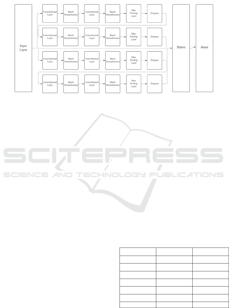
Figure 1: Architecture of model (Picture credit : Original)

2.3 Optimizations

The model contains three main optimization methods,

dropout, early stopping, and Gradient descent which

are used to reduce the time of training as well as

improve accuracy.

During training, a portion of the input units are

randomly dropped as part of the dropout optimization

technique, which aims to prevent overfitting. In the

model, the dropout has an increasing chance of

dropping a neuron per layer, from a 20% rate in the

first dropout layer to 50% in the last with steps of

10%, which makes the dropped neuron not contribute

to the result. This is beneficial as this allows neurons

to learn without dependence on other neurons.

Early stopping is an algorithm that stops the

training process early when little is changed in the

model’s weights and values to prevent overfitting as

well as improve the time efficiency of the model, as

the training time is reduced. Early stopping consists

of a patience value, which is the number of epochs the

model waits before early stopping happens.

Stochastic gradient descent (SGD), a technique

for locating local minima of parameter loss, is also

used in the model. This is accomplished by

computing the partial derivatives to update the

parameters and determining the gradient of the loss

function with respect to each parameter. Every epoch,

this process is carried out again until convergence

(local minimum of loss) is achieved. The model

employs a particular gradient descent technique based

on the Adam algorithm, which reduces memory

consumption and enhances performance by taking

into account both adaptive learning rates to handle

changing data and the exponentially weighted

average to find the minimum more quickly.

3 RESULTS

Results are measured using the validation dataset of

the images, where the model has not seen these

images before. The performance of the model is

tested on its accuracy and its loss. The experiment

was carried out on a Mac computer with a m2 CPU

and 16GB of memory, with a total training time of 4

hours 50 minutes.

The model is early stopped at epoch 273 with little

change in its parameters. Results show a 91.14%

accuracy and a loss of 0.4014 on the testing data in

the final epoch, as shown in Table 1.

Table 1: Loss and accuracy of epoch

Epoch Loss Accuracy

1 1.701 0.422

50 0.638 0.858

100 0.481 0.892

150 0.42 0.903

200 0.401 0.911

250 0.404 0.910

273 0.401 0.912

Using Neural Networks to Build an Efﬁcient Classiﬁcation Model for Classifying Images in the CIFAR-10 Dataset

151

Figure 2 is loss per epoch. The observation that

both training and validation loss curves exhibit a

gradual decline with the increasing number of

training epochs is a common trend in the training

process of machine learning models. This pattern

indicates that the model is learning and improving its

ability to fit the training data. The fact that the losses

reach their minimum at the 250th epoch suggests that

the model has been adequately trained and has found

a set of weights that provide a good balance between

fitting the training data and not overfitting to it. The

training and validation loss curves are essential for

visualizing the model's learning process. The training

loss typically decreases as the model learns the

patterns in the training data. The validation loss,

which is computed on a separate set of data not used

in training, provides an estimate of the model's

performance on unseen data.

Figure 2: Loss per epoch (Picture credit : Original)

Figure 3 is accuracy per Epoch. It can be seen that

the training loss and the validation loss show a

gradual increase trend with the increase of epochs,

and reach the maximum accuracy at 250 epochs. So

this training process is valid.

Figure 3: Accuracy per epoch (Picture credit : Original)

4 CONCLUSIONS

In this work, a CNN model for classifying images into

ten groups using the CIFAR-10 dataset is developed.

Eight convolutional layers, eight batch normalisation

layers, four max-pooling layers, and dropout layers

are sandwiched between every two convolution and

batch normalisation levels in this CNN model

architecture. In order to further reduce training time

and improve performance by preventing overfitting,

the model additionally employs early stopping. When

the program is backpropagated, the Adam optimizer

method allows faster and better memory usage when

minimizing the loss function. When trained, a result

of 91.14% accuracy shows that this model can

accurately classify images into its classes. The model

have many improvements by increasing the number

of layers, which could lead to improved accuracy but

increases complexity as well as risk to overfitting. In

the future, with more efficient and accurate

algorithms, image classification could reach new

accuracy and greater efficiency levels.

REFERENCES

Abiodun, O. I., Jantan, A., Omolara, A. E., Dada, K. V., Mo

Mohamed, N. A., & Arshad, H. (2018). State-of-the-art

in artificial neural network applications: A survey.

Heliyon, 4(11).

Wu, J. (2017). Introduction to convolutional neural

networks. National Key Lab for Novel Software

Technology. Nanjing University. China, 5(23), 495.

Cai, S., Shu, Y., Chen, G., Ooi, B. C., Wang, W., & Zhang,

M. (2019). Effective and efficient dropout for deep

convolutional neural networks.

Kingma, D. P., & Ba, J. (2014). Adam: A method for

stochastic optimization.

Krizhevsky, A. (2009). Learning Multiple Layers of

Features from Tiny Images.

Krizhevsky, A., & Hinton, G. (2010). Convolutional deep

belief networks on cifar-10. Unpublished manuscript,

40(7), 1-9.

Krizhevsky, A., Sutskever, I., & Hinton, G. E. (2012).

Imagenet classification with deep convolutional neural

networks. Advances in neural information processing

systems, 25.

LeCun, Y., Bottou, L., Bengio, Y., & Haffner, P. (1998).

Gradient-based learning applied to document

recognition. Proceedings of the IEEE, 86(11), 2278-

2324.

Lei, X., Pan, H., & Huang, X. (2019). A dilated CNN model

for image classification. IEEE Access, 7, 124087–

124095.

Prechelt, L. (2002). Early stopping-but when?. In Neural

Networks: Tricks of the trade (pp. 55-69). Berlin,

Heidelberg: Springer Berlin Heidelberg.

DAML 2024 - International Conference on Data Analysis and Machine Learning

152

Simonyan, K., & Zisserman, A. (2014). Very deep

convolutional networks for large-scale image

recognition. arXiv preprint arXiv:1409.1556.

Taylor, L., & Nitschke, G. (2017). Improving deep learning

using generic data augmentation.

Using Neural Networks to Build an Efﬁcient Classiﬁcation Model for Classifying Images in the CIFAR-10 Dataset

153