Flower Pictures Recognition Based on the Advanced Convolutional

Neural Network with Oxford Flowers 102 Dataset

Jiarui Hu

Shoreline Community College, Seattle, U.S.A.

Keywords: Flower Recognition, CNN, Oxford Flowers 102 Dataset, Deep Learning.

Abstract: This paper established a model and trained it to recognize pictures of 102 types of oxford flowers by using

Convolutional Neural Network (CNN) Because enhancing effectiveness and efficiency while reducing labor

costs is the main advantage of autonomic flower classification technology. This study employs the Oxford

Flowers 102 dataset and performs a series of random transformations and adjustments in data preparation.

The model consists of convolutional layers (extracts local features by convolving kernels with input images),

pooling layers (reduces resolution and parameters), and fully connected layers (combines and classifies

features) are employed. Besides, a sequential model is created using tf.keras. Sequential class. It contains

multiple max pooling layers, one global average pooling layer, three fully connected layers with Rectified

Linear Unit (ReLU) activation and L2 regularization along with Dropout layers, and four convolutional layers

with different numbers of filters. Eventually it achieves about 70% accuracy in recognizing flower pictures.

8 versions of the model are carried out to construct a better one. The further study plans involve continuous

learning and adaptation by exploring more advanced technology and parameters to become more proficient

in this field.

1 INTRODUCTION

Flowers are the propagative organs of angiosperms.

They often grow with vivid color, special shape,

luscious smell and sweet nectar to attract pollinators

like butterflies and bees. Most places with sunlight,

minerals, air and water can be the probable growing

environments. Flowers are vital to both the natural

world and human life. In nature, the significant

importance of flowers reflected in multiple aspects:

Their reproduction can help maintain the ecological

balance and promote the formation of biodiversity;

They participate in the mineral circulation and energy

flow of the ecosystem; They provide food resource

for various animals. For humans, flowers possess

commercial, artistic, medicinal value and symbolic

meaning.

Flower classification is widely used in wild

scientific research, flower selling, horticulture and

agriculture, bontany education, Cultural inheritance

and communication (Nilsback, 2008; Nilsback, 2006;

Hiary, 2018; Xia, 2017). However, traditional

methods of flower classification rely heavily on

https://orcid.org/0009-0004-2951-925X

human labor. Experts and botanists painstakingly

examine various characteristics of flowers, such as

petal shape, color, size, and the structure of

reproductive organs. This process is not only time-

consuming but also prone to errors due to human

fatigue and subjectivity. The low efficiency of

manual classification limits the scale and speed of

flower identification and research.

Autonomic classifying flowers technology can

improve effectiveness and efficiency as well as

reduce labor cost. It possesses remarkable capabilities

in feature extraction. Through advanced algorithms

and machine learning techniques, artificial

intelligence can analyze large amounts of data and

identify subtle and complex features that might be

overlooked by the human eye. Therefore, this

research direction deserves more attention.

Artificial Intelligence (AI) has a long and

fascinating development history (Hunt, 2014;

Holzinger, 2019; Fetzer, 1990). Over the years, it has

evolved from simple rule-based systems to

sophisticated machine learning and deep learning

models. The trend in artificial intelligence is towards

336

Hu, J.

Flower Pictures Recognition Based on the Advanced Convolutional Neural Network with Oxford Flowers 102 Dataset.

DOI: 10.5220/0013330800004558

Paper published under CC license (CC BY-NC-ND 4.0)

In Proceedings of the 1st International Conference on Modern Logistics and Supply Chain Management (MLSCM 2024), pages 336-341

ISBN: 978-989-758-738-2

greater automation, accuracy, and adaptability.

Representative algorithms play a crucial role in this

evolution. Random forests and decision trees are

classical machine learning algorithms. Random

forests combine multiple decision trees to improve

prediction accuracy and reduce overfitting. Decision

trees, on the other hand, use a hierarchical structure to

make decisions based on features of the data. Neural

networks, especially deep neural networks, have

revolutionized the field of artificial intelligence. They

can learn complex patterns and relationships in data

and have achieved remarkable results in various

tasks.

Among them, Convolutional Neural Networks

(CNN) have emerged as the dominant algorithm in

computer vision. CNNs are designed to process grid-

like data such as images and have shown exceptional

performance in tasks like image classification, object

detection, and segmentation. Their success has led to

their widespread application in multiple fields. In

chemistry, CNNs have been used for predicting

molecular properties and drug design. In biology,

they have been applied to analyze biological images

and sequences. In medicine, they are utilized for

medical image analysis and disease diagnosis. In

agriculture, there are numerous applications. For

example, some researchers have used specific

algorithms to predict tree classification and leaf

classification, helping in tasks such as disease

detection in plants and yield prediction.

Given the proven effectiveness of AI in these

diverse fields, this paper aims to leverage AI,

particularly CNN technology, for predicting flower

classification. This approach not only has the

potential to improve the accuracy of flower

classification but also offers a more intuitive way to

understand and interpret the results.

This article uses the dataset from tensorflow. This

study erects a model with four convolutional layers

and focus on visual analysis. Visual analysis

involves: Plotting the accuracy and loss curves on the

training set and validation set to observe the learning

trend of the model; For some test images, showing the

prediction results of the model and comparing them

with the true labels.

2 METHOD

2.1 Data Preparation

For dataset preparation, this paper uses the Oxford

Flowers 102 dataset (Nilsback, 2008), which is from

website Tensorflow. The size of the single image is

not uniform, requiring further processing. The

dataset consists of 102 flower categories generally

occurring in the United Kingdom. There are 40 to 258

images in each class. The images have huge scale,

light variations and pose. Also, there are categories

that exhibit significant variations within the category

itself, and several categories that are very similar to

each other.

The dataset is divided into three sets: a training

set, a validation set and a test set. The training set and

validation set both comprise 10 images per class each

(totaling 1, 020 images respectively). The test set is

made up of the remaining 6, 149 images (with a

minimum of 20 per class), as shown in the following

figure. The following Figure 1 shows some examples

of images and their corresponding labels.

Figure 1: The sample images used in this study (Nilsback,

2008).

In this study, each image is resized into a square with

a length of 200 pixels. The image enhancement

function of TensorFlow is used to perform a series of

random transformations on images, including left-

right flipping, up-down flipping, contrast adjustment,

brightness adjustment, saturation adjustment, and hue

adjustment.

2.2 Convolutional Neural Network

CNN is a kind of deep learning model, widely used in

image recognition, speech recognition, and other

fields (Gu, 2018; Yamashita, 2018; Wu, 2017). The

core idea of CNN is to reduce the number of

parameters and improve the efficiency and

generalization ability of the model through local

perception and weight sharing. Local perception

means that each neuron is only connected to a local

area of the input image to extract local features.

Weight sharing refers to the use of the same

convolution kernel by multiple neurons in the same

layer, thereby reducing the number of parameters.

Flower Pictures Recognition Based on the Advanced Convolutional Neural Network with Oxford Flowers 102 Dataset

337

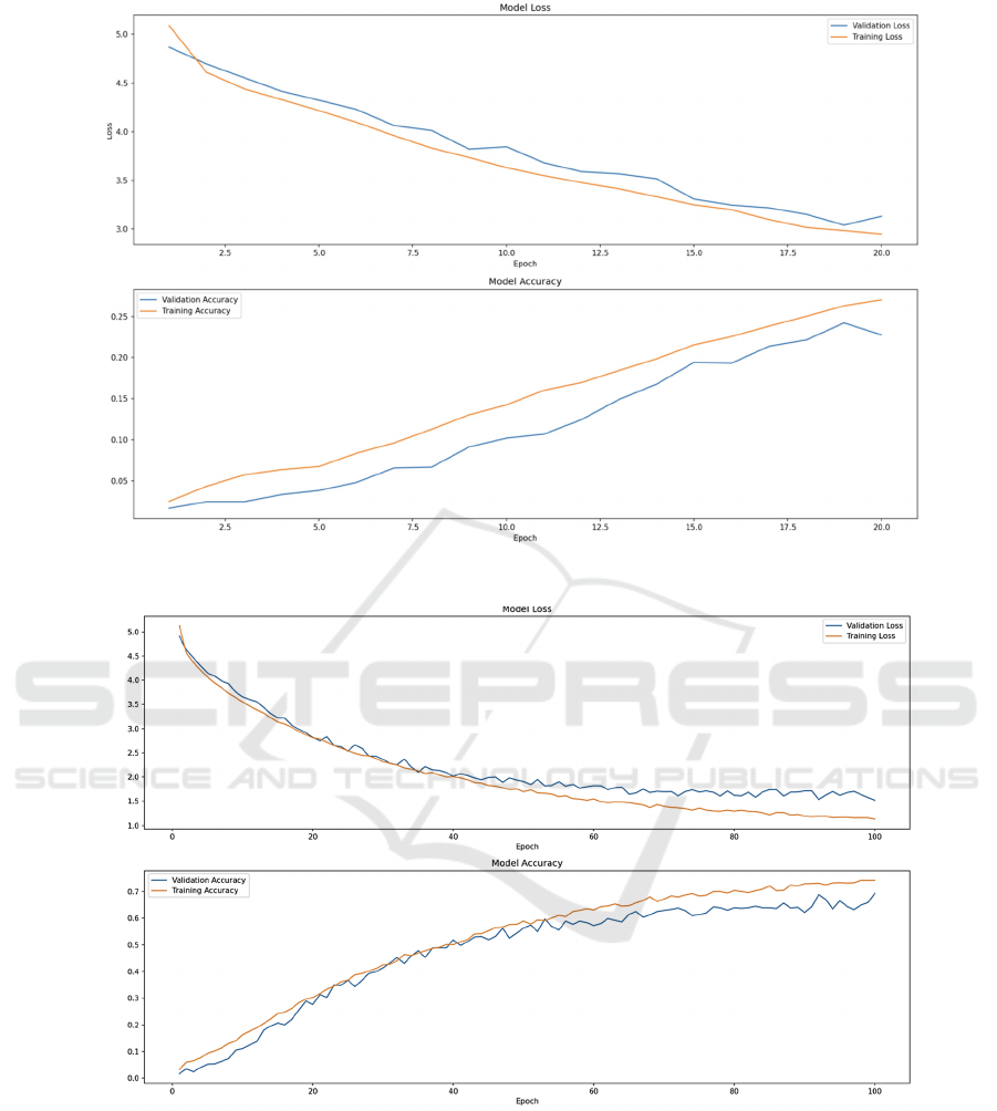
Figure 2: The performance of the model-1 (Photo/Picture credit: Original).

Figure 3: The performance of the model-2 (Photo/Picture credit: Original).

It includes three modules: convolutional Layer,

pooling layer and fully connected layer. The

convolutional layer is the main part of CNN, which

extracts the local features of the images by

convolving the convolution kernels with the input

images. The convolution kernel can be regarded as a

filter that can detect specific patterns and features in

the image. The size and number of convolution

kernels can be adjusted according to needs. By

adjusting the size, number, and parameters of the

convolution kernel, features of different levels and

types can be extracted. After more extraction times of

images, the extracted feature maps from

convolutional layer become more abstracted. The

pooling layer is used to reduce the resolution of the

feature map, reduce the number of parameters and

MLSCM 2024 - International Conference on Modern Logistics and Supply Chain Management

338

computational costs. This paper contains max pooling

and global average pooling. Both of them are

common pooling operations. The fully connected

layer combines and classifies the features extracted

by the convolutional and pooling layers. It connects

all neurons of this current layer to all neurons in the

previous layer to achieve comprehensive analysis and

judgment of the features. The fully connected layer is

usually used in the last few layers of CNN to output

the classification result or prediction value.

Inside the function of model part, a sequential

model is created by using the tf.keras.Sequential

class. The model contains three max pooling layers,

one global average pooling layers, three fully

connected layers, two Dropout layers, and four

convolutional layers. To be specific, the model

structure constructs as can be seen below:

The first layer is a convolutional layer with 32

filters: kernel size is (3, 3), the activation method is

ReLU, and input shape is (200, 200, 3). The second

max pooling layer contains a (2, 2) pool size. The

third layer is a convolutional layer with 64 filters. The

kernel size is still (3, 3) and the activation function is

still ReLU. These components except the number of

filters are not going to change for every convolutional

layer. The fourth layer is the same as the second one.

Then there are two convolutional layers with 128 and

256 filters respectively. After that is the same max

pooling layer as well. Then there is a global average

pooling layer. After that are two fully connected

layers with 256 and 128 neurons respectively. The

activation function is Rectified Linear Unit (ReLU),

and L2 regularization are both used in two fully

connected layers. Behind each fully connected layer

is a Dropout layer with a dropout rate of 0.5. Finally,

there is an output layer with 102 neurons and the

activation function is softmax.

2.3 Implementation Details

This experiment is implemented through tensorflow.

When compile the model, the optimizer is set

as Adam. In deep learning, an optimizer is used to

adjust the parameters of a model in order to minimize

the loss function. When training the model, this study

uses 100 epochs as training time number. In machine

learning and deep learning, an evaluation metric is a

measure used to assess the performance of a model.

3 RESULTS AND DISCUSSION

This study tries to build several versions of the model

for aiming higher accuracy. On the Figure 2 above,

the upper one represents the training history of the

loss of model of version 5, and the lower one

represents the accuracy of model. This figure is the

version of 20 epochs training. This figure shows the

evaluation results of the model while training. As

shown in the Figure 3 above, the x-axis labels the

times of epoch, and the y-axis represents the value of

loss and accuracy. The loss rates decrease over time,

while the accuracy rates increase. Training loss

measures the percentage of incorrect interpretation on

the training dataset, and validation loss evaluates the

performance of the model on a separate validation

dataset. The training loss descends from about 5.1 to

2.9, and the validation loss decreases from about 4.9

to 3.2. Vice versa, for training accuracy demonstrates

how well the model is learning on the training dataset,

while validation accuracy gives an indication of the

model's ability to generalize to new dataset given.

Training accuracy ascends from about 2% to 27%,

and validation accuracy increases from about 1% to

23%.

After 100 epochs of training of the model, the loss

and accuracy changes more drastically than just 20

epochs. The training loss cuts down to about 1.2, and

the validation loss reduces to about 1.5. The

differences between the formers and the later are

about 1.7. In turn, training accuracy is up to about

77%, and validation accuracy adds to about 69%.

Therefore, the accuracies grow 50% and 46% for the

following 80 epochs.

Firstly, random adjustments were made to the data

in the pre-processing part, and then the parameters

and layers of the model were adjusted and several

regularizers were added to build up this accuracy.

Afterwards, this study tries to improve the

performance of the model by increasing the

complexity of it and altering the parameters to

achieve a higher accuracy, which corresponds to the

later versions 6 and 7. However, the accuracy of these

two versions was only around 0.65, which was lower

than that of version 5. Therefore, version 5 was

ultimately selected. The sample size is insufficient to

support higher accuracy. After all, there are only

8,200 samples to be trained to recognize 102 flowers

and part of these samples have to be separated into

test dataset and validation dataset. This paper may

need to import some pre-trained models to be more

accurate.

Besides, the model training takes a long time. The

efficiency of the model still needs to be improved.

There are several probable methods to improve the

speed of model training: Changing the electronic

devices that were used, and using a more powerful

hardware; Optimizing the model architecture. Like,

Flower Pictures Recognition Based on the Advanced Convolutional Neural Network with Oxford Flowers 102 Dataset

339

reducing the complexity of the model by reducing the

number of parameters or using more efficient

architectures. However, this means affect the

accuracy rates of the result; Reducing the number of

epochs, but it sacrifices model performance too.

The variation in flower features is likely

influenced by factors such as genetic mutations,

growth conditions, and growth stages, all of which

can affect their appearance and make identification

more challenging.

Figure 4: The Feature Map and Label Prediction-1

(Photo/Picture credit: Original).

For some test images, these are prediction results of

the model and compare them with the true labels. On

the three pictures above, the left schematic diagrams

are the feature maps extracted by the model. Under

they are the true labels and in parentheses are the

labels predicted by the model. Then on the right side

of each picture are the proportion of each label for this

flower in the picture. Figure 4 are the results after

training the model for 10 epochs. And Figure 5 are

the results after 30 epochs training.

Figure 5: The Feature Map and Label Prediction-2 (Photo/

Picture credit: Original).

4 CONCLUSIONS

This article uses the CNN technology in AI deep

learning algorithm region to learn the pictures of 102

kinds of flowers in oxford and completes the task of

recognizing flower pictures with an accuracy rate of

up to about 70%. A series of random transformations,

contrast adjustment, brightness adjustment, saturation

adjustment, and hue adjustment are applied to images

while pre-processing the data. Extensive experiments

were conducted to construct more effective and

efficient models to identify pictures. In the future, the

further study plans to learn and adapt continuously to

become more proficient in this field by exploring

more advanced technology and parameters.

REFERENCES

Fetzer, J. H., & Fetzer, J. H. 1990. What is artificial

intelligence? (pp. 3-27). Springer Netherlands.

Gu, J., Wang, Z., Kuen, J., Ma, L., Shahroudy, A., Shuai,

B., ... & Chen, T. 2018. Recent advances in

convolutional neural networks. Pattern recognition, 77,

354-377.

Hiary, H., Saadeh, H., Saadeh, M., & Yaqub, M. 2018.

Flower classification using deep convolutional neural

networks. IET computer vision, 12(6), 855-862.

Holzinger, A., Langs, G., Denk, H., Zatloukal, K., &

Müller, H. 2019. Causability and explainability of

artificial intelligence in medicine. Wiley

MLSCM 2024 - International Conference on Modern Logistics and Supply Chain Management

340

Interdisciplinary Reviews: Data Mining and

Knowledge Discovery, 9(4), e1312.

Hunt, E. B. 2014. Artificial intelligence. Academic Press.

Nilsback, M. E., & Zisserman, A. 2008. Automated flower

classification over a large number of classes. In 2008

Sixth Indian conf. on computer vision, graphics &

image processing (pp. 722-729). IEEE.

Nilsback, M. E., & Zisserman, A. 2006. A visual

vocabulary for flower classification. In 2006 IEEE

computer society conference on computer vision and

pattern recognition (CVPR'06) (Vol. 2, pp. 1447-1454).

IEEE.

Wu, J. 2017. Introduction to convolutional neural networks.

National Key Lab for Novel Software Technology.

Nanjing University. China, 5(23), 495.

Xia, X., Xu, C., & Nan, B. 2017. Inception-v3 for flower

classification. In 2017 2

International Conf. on image,

vision and computing (ICIVC) (pp. 783-787). IEEE.

Yamashita, R., Nishio, M., Do, R. K. G., & Togashi, K.

2018. Convolutional neural networks: an overview and

application in radiology. Insights into imaging, 9, 611-

629.

Flower Pictures Recognition Based on the Advanced Convolutional Neural Network with Oxford Flowers 102 Dataset

341