Implementation of Artificial Intelligence Algorithms in Brain Tumor

Detection and Classification

Lizhuo Xu

Shanghai Datong High School, Shanghai, China

Keywords: Artificial Intelligence, Medical, Brain Tumor, Convolutional Neural Network.

Abstract: Brain tumors in the early stage are difficult to detect and doctors may misdiagnose due to many reasons, such

as tiredness, insufficient experience, or maybe even just carelessness. Artificial intelligence (AI) algorithms

can be used to help doctors diagnose. This study developed a model that identifies and classifies three types

of brain tumors using Magnetic Resonance Imaging (MRI) images. This study used a dataset from Kaggle.

The chosen dataset was preprocessed by first creating a validation set from the original training set. Data

augmentations like brightness changing, saturation changing, and contrast changing were used. Images in the

dataset were also randomly flipped. The model developed by this study used the Convolutional Neural

Network (CNN) technology. Transfer learning was used in this study to promote the feature extraction ability

of the model. The pre-trained model VGG19 was used as the base model. A convolutional layer and several

fully connected layers were used after the base model. Dropout layer and regularizers were added to prevent

potential overfitting. After training, the model showed a relatively good test performance and indicates that

artificial intelligence algorithms have great potential in the task of detecting and classifying brain tumors

using MRI images.

1 INTRODUCTION

A tumor is an abnormal growth of cells in a certain

part of the human body. Tumors are caused by

multiple factors e.g. genetic factors, unhealthy

lifestyles, environmental factors etc. Tumors may

even grow with unknown factors. Brain tumors are a

specific kind of tumors that grows around the human

brain area. They can cause great danger to the human

body. For example, brain tumors may cause mental

disorders, diminution of vision, headaches, and many

other symptoms (Madhusoodanan, 2015; Jarquin-

Valdivia, 2004). Just like other tumors, severe brain

tumors may eventually turn into cancer, which is one

of the main causes of natural death today. Therefore,

it is crucial to prevent the progression of brain tumors.

A key factor in preventing the progression of brain

tumors is early detection. The earlier the tumors are

detected, the sooner the treatment can begin and this

can reduce the probability of potential deterioration

of the tumors. One of the most common ways of

detecting tumor growth is analyzing Magnetic

Resonance Imaging (MRI) images. Traditionally,

https://orcid.org/0009-0002-1551-1527

doctors need to look over the MRI images by

themselves to check whether there is a tumor or not

based on their own experience. This may lead to some

potential problems. For example, tumors in the early

stage are usually relatively small and hard to detect.

Besides this, the doctor may make a careless mistake

due to tiredness or some other random reasons, and

misdiagnoses will happen in some situations. The

Artificial Intelligence (AI) technology that develops

rapidly these days may be an ideal choice to assist

doctors in diagnoses. The combination of the

powerful feature extraction capability of AI

algorithms and the experience and judgment of the

human doctor can help diagnose more precisely.

Different kinds of widely used AI techniques were

proposed these years, such as Convolutional Neural

Networks (CNNs), Decision Trees, Random Forests

etc. Those algorithms have been applied to a broad

range of fields. For instance, in the physics field,

Hennigh et al. presented an AI-driven multi-physics

simulation framework, SimNet, to accelerate science

and engineering simulations (Hennigh, 2021). AI

techniques are also used in the chemical field. For

Xu, L.

Implementation of Artiﬁcial Intelligence Algorithms in Brain Tumor Detection and Classiﬁcation.

DOI: 10.5220/0013281300004558

In Proceedings of the 1st International Conference on Modern Logistics and Supply Chain Management (MLSCM 2024), pages 219-223

ISBN: 978-989-758-738-2

219

example, Cho et al. examined the possibility of using

deep neural network to enhance gas sensing below the

limit of detection region to get more information

about the object (Cho, 2020). Furthermore, in the

medical field, AI techniques are useful as well. Levy

et al. conducted a study to evaluate the performance

of AI in the interpretation of focused assessment with

sonography in trauma (FAST) examination

abdominal views and concluded that AI is a feasible

approach to improve imaging interpretation accuracy

(Levy, 2023). As for the implementation of AI in

brain tumor detection, some researchers have

conducted researches on this topic before as well.

Almadhoun et al. used deep learning techniques to

design a model and test the performance of different

models in finishing this task (Almadhoun, 2022).

Hemanth et al. used techniques of machine learning

and data mining to explore the implementation of AI

in the task (Hemanth, 2019).

Considering the significance of this field, this

study aims to use AI algorithms to develop a model

that can help identify three main types of brain tumors

(i.e. Pituitary Tumors, Meningiomas, and Gliomas).

The specific technique used in this study is CNN. The

dataset used in this study is the Kaggle dataset “Brain

Tumor Classification (MRI)” which includes 3,264

MRI images of three main types of brain tumors and

no-tumor ones. This study altered the parameters and

the structure of the developed model to investigate the

performance of the CNN model in the brain tumor

classification task.

2 METHOD

2.1 Dataset Preparation

This study uses the dataset “Brain Tumor

Classification (MRI)” from Kaggle, which includes

3,264 images in total (Kaggle, 2020). Those images

in the dataset are on the RGB scale with various

image sizes. The dataset consists of four different

classes: “glioma_tumor”, “meningioma_tumor”,

“pituitary_tumor”, and “no_tumor” corresponding to

MRI images of glioma tumor patients, meningioma

tumor patients, pituitary tumor patients, and patients

with no tumor. The dataset has an original split of 394

images for testing and 2,870 images for training. Each

split includes images from all four classes.

After downloading the dataset from Kaggle and

extracting the file, this study loaded the dataset in the

memory. The testing set and the training set were

loaded separately. All sample images were loaded in

a size of 300 pixels by 300 pixels and preserved on

the RGB scale. This study reorganized the dataset

split to create a validation dataset for tracking the

model performance during the training progress. The

validation set was created from the shuffled training

set of the original split. The final split of the dataset

was 2,583 samples for the training set, 287 samples

in the validation set, and 394 samples in the testing

set. This study also employed some data

augmentation methods to help the model learn better

since the size of the chosen dataset cannot be

considered large. The contrast, brightness, and

saturation of sample images were randomly altered.

The contrast and the saturation were both set with an

upper bound of 1.3 and a lower bound of 0.7. The

brightness change was set with a max delta, which

means the max change, of 0.3. The sample images

were also randomly flipped left right and randomly

flipped up down. All three sets, training, validation,

and testing, were batched in a batch size of 32. The

reorganized dataset was prefetched. The prefetch

buffer size of the dataset is determined automatically,

to improve the efficiency of computation.

2.2 Convolutional Neural Network-

Based Prediction

This study used a CNN model. CNN is a type of

Neural Network (NN) that is mainly used to process

images or other kinds of grid-form data (Gu, 2018;

Yamashita, 2018). A CNN usually contains

convolutional (Conv) layers, pooling layers, and fully

connected (FC) layers. The FC layers can also be

called dense layers. The use of convolutional layers

in the model is the main difference between CNNs

and NNs. Filters are used in Conv layers to scan

through the input and generate feature maps

according to the result obtained from the scanning.

Those filters are also called kernels. The pooling

layers are another important kind of layer in a CNN

model. The input spatial dimension can be reduced by

using this kind of layer. Doing this has several

benefits, such as preventing possible overfitting,

helping the model to summarize, and reducing the

computation load. Pooling layers have several types,

like max pooling layers and global average pooling

layers. Global pooling layers are typically used

between the convolutional part and the fully

connected part of the model to connect those two

parts. Ordinary pooling layers are usually used after a

Conv layer or a block of Conv layers. The FC layers

are a kind of layer that consists of neurons. Each

neuron in this kind of layer is connected to every

neuron in the previous layer. This kind of layer can

be used to increase the complexity of the model or as

MLSCM 2024 - International Conference on Modern Logistics and Supply Chain Management

220

the output layer. Another essential component of the

model is the activation function. All those Conv

layers and FC layers need activation functions. Some

common choices are Rectified Linear Unit (ReLU),

Sigmoid, and Softmax.

The model developed by this study uses transfer

learning to improve the feature extraction ability. The

pre-trained model used as the base model in this study

is VGG19, which is a model that has strong

generalization capability. Only the convolutional

blocks were preserved when loading VGG19 as the

base model. This study used the weights that the pre-

trained model learned from the training on the

“ImageNet” dataset and set the base model

untrainable, which means that the weights of the base

model would not be changed during the training

progress. This study added one more Conv layer after

the base model. This layer has 128 kernels with a

kernel size of 3 by 3. This layer uses Swish as the

activation function. This layer is followed by a max

pooling layer with a pooling window size of 2 by 2.

This study used a global average pooling layer as the

connection between the convolutional and fully

connected parts of the model. Six FC layers,

including the one for output, were used after the

global average pooling layer. The numbers of units,

which means the number of neurons in that layer, of

those FC layers were set to be 128, 64, 32, 16, 8, and

4, from the first FC layer to the last one

correspondingly. The first five FC layers all use

Swish as the activation function. The activation

function Softmax is used in the last FC layer. This FC

layer is used as the output layer in this model. In order

to prevent potential overfitting, right after each of the

first, second, and third FC layers, a dropout layer with

a dropout rate of 0.5 was added. A kernel regularizer

using an L2 regularizer with a regularization strength

of 0.001 was added to each of the second, third, and

fourth FC layers.

2.3 Implementation Details

This study used TensorFlow to build the model. The

optimizer used by this study was Adaptive Moment

Estimation (Adam), which can adapt the learning

rates for parameters dynamically. The model was

trained for 60 epochs. Two early stoppings were set

with metrics of validation loss and validation

accuracy and were both set with a patience of 50

epochs. The early stopping for validation loss was set

to restore the weights of the model in the epoch that

had the best performance in validation loss. However,

during the training, the early stoppings were never

triggered and the model trained for all 60 epochs. This

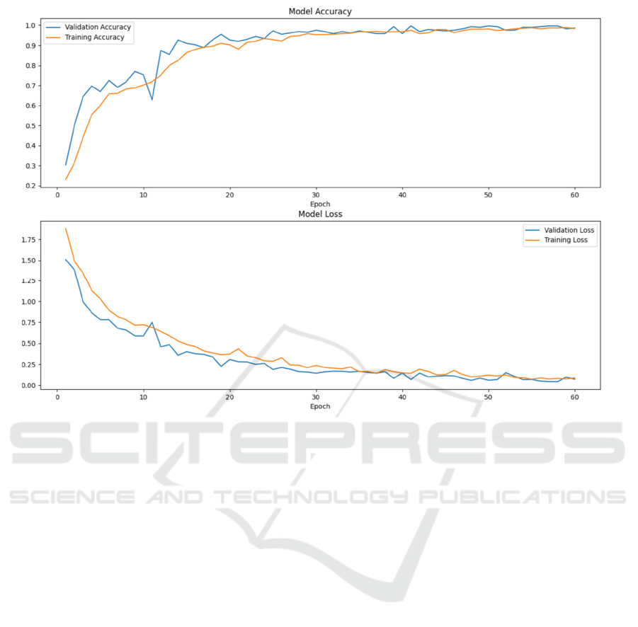
Figure 1: Training curve of the model developed by this study (Photo/Picture credit: Original).

Implementation of Artiﬁcial Intelligence Algorithms in Brain Tumor Detection and Classiﬁcation

221

study chose the Sparse Categorical Crossentropy

Loss as the loss function and ‘accuracy’ as the

evaluation metric.

3 RESULTS AND DISCUSSION

The model developed by this study was trained and

tested. Its training curve is shown in Figure 1 and the

training, validation, and testing performance is shown

in Table 1.

According to the training curve in Figure 1, it can

be discovered that the increasing speed of accuracy

and the decreasing speed of loss slow down to almost

stop at the end of the 60–epoch training. As a result,

it does not seem likely that the performance of the

model could be promoted significantly by increasing

the epoch number.

From the training, validation, and testing results

in Table 1, it can be found that the model achieved

high accuracies on both the training set and the

validation set after finishing all 60 epochs of training.

The final training loss and validation loss are low.

Although the final test accuracy is not high enough

for direct implementation in the medical field, it still

shows the great potential of AI algorithms in

identifying brain tumors and classifying their types

using MRI images.

Although according to both Table 1 and Figure 1,

the validation and training accuracy curves fit each

other relatively well and show high accuracies and

low losses at the end of the training, a difference of

about 0.18 is shown between the accuracies of the last

epoch, both the training one and the validation one,

and the final test accuracy. The final test accuracy is

lower. The final test loss also turned out to be higher

than the training loss and the validation loss at the end

of the training progress. There are two possible causes

for this problem. The first one is that the model may

be overfitting to the validation set and the training set.

Another potential reason is the distribution difference

in the difficulty of the training set and the testing set

from the original split. The validation set used in this

study was split from the training set of the original

split, so a distribution difference in the difficulty of

the training and testing set of the original split may

lead to this problem. A training dataset with a larger

size and more diverse data may help further promote

the performance of the model since the dataset used

by this study cannot be considered as a large dataset

and the MRI images in it are taken from different

angles.

Table 1: The training and testing results of the model

developed by this study.

Model Trainin

Accura

cy*

Traini

Loss*

Validat

ion

Accura

cy*

Validat

ion

Loss*

Test

Accur

acy

Test

Loss

The

model

develo

ped by

this

stud

0.9845 0.081

0.9861 0.0704 0.8046 1.95

*: Obtained in the last training epoch.

4 CONCLUSIONS

In this study, a brain tumor identification and

classification model using CNN combined with

transfer learning was designed. The model uses a pre-

trained model as a base model to promote the feature

extraction ability. The model was trained and tested

using the dataset. The model showed a relatively good

test result which showed the potential of AI

algorithms in detecting brain tumors and classifying

their types. AI algorithms have great potential in

helping doctors analyze MRI images and make

diagnoses. However, the performance of the model

may be further promoted. The dataset used in this

study is not large and there seems to have a

distribution difference in the difficulty of the original

training set and the original testing set. With more

training data and some further modifications to the

model, the model may be able to achieve a better

performance in this task. In the future, the further

study plans to continue to explore the application of

AI algorithms in this field and try to develop a model

with a better performance.

REFERENCES

Almadhoun, H. R., & Abu-Naser, S. S. 2022. Detection of

brain tumor using deep learning. International Journal

of Academic Engineering Research (IJAER), 6(3), 29-

47. https://philpapers.org/rec/ALMDOB

Cho, S. Y., Lee, Y., Lee, S., Kang, H., Kim, J., Choi, J.,

Ryu, J., Joo, H., Jung, H. T., & Kim, J. 2020. Finding

hidden signals in chemical sensors using deep learning.

Analytical Chemistry, 92(9), 6529-6537.

Gu, J., Wang, Z., Kuen, J., Ma, L., Shahroudy, A., Shuai,

B., ... & Chen, T. 2018. Recent advances in

convolutional neural networks. Pattern recognition, 77,

354-377.

MLSCM 2024 - International Conference on Modern Logistics and Supply Chain Management

222

Hemanth, G., Janardhan, M., & Sujihelen, L. 2019. Design

and implementing brain tumor detection using machine

learning approach. In 2019 3rd International

Conference on Trends in Electronics and Informatics

(ICOEI) (pp. 1289-1294). IEEE.

Hennigh, O., Paszynski, M., Kranzlmüller, D.,

Krzhizhanovskaya, V. V., Dongarra, J. J., & Sloot, P.

M. 2021. NVIDIA SimNet™: An AI-accelerated multi-

physics simulation framework. Computational science

– ICCS 2021 (Vol. 12746). Springer.

Jarquin-Valdivia, A. A. 2004. Psychiatric symptoms and

brain tumors: a brief historical overview. Archives of

Neurology, 61(11), 1800-1804.

Kaggle. 2020. Brain tumor classification MRI.

https://www.kaggle.com/datasets/sartajbhuvaji/brain-

tumor-classification-mri

Levy, B. E., Castle, J. T., Virodov, A., Wilt, W. S.,

Bumgardner, C., Brim, T., McAtee, E., Schellenberg,

M., Inaba, K., & Warriner, Z. D. 2023. Artificial

intelligence evaluation of focused assessment with

sonography in trauma. Journal of Trauma and Acute

Care Surgery, 95(5), 706-712.

Madhusoodanan, S., Ting, M. B., Farah, T., & Ugur, U.

2015. Psychiatric aspects of brain tumors: a

review. World journal of psychiatry, 5(3), 273.

Yamashita, R., Nishio, M., Do, R. K. G., & Togashi, K.

2018. Convolutional neural networks: an overview and

application in radiology. Insights into imaging, 9, 611-

629.

Implementation of Artiﬁcial Intelligence Algorithms in Brain Tumor Detection and Classiﬁcation

223