Investor’s View Adjustment of Black Litterman Model Based on

LSTM Recurrent Neural Network

Guanyun Ding

Beijing Royal School, Beijing, China

Keywords: LSTM Recurrent Neural Network, Black Litterman Model, Portfolio Management, Machine Learning

Algorithm, Mean-Variance Approach.

Abstract: As a matter of fact, managing assets by considering investors' expectations and goals is essential in portfolio

management. Many other researchers changed the method after Fischer Black and Robert Litterman raised

the idea of combining investors' views with market equilibrium returns. They applied machine learning

technology to provide a new route for further portfolio management development. This study evaluates a

convenient way to adjust investors' views in the Black Litterman model using an LSTM (Long Short-Term

Memory) recurrent neural network. Several LSTM(1d) models have been built to forecast the asset price trend,

and for example, the investor's view is adjusted using the model's projection. Furthermore, the result of the

traditional BL model is compared with the LSTM adjusted model. Results show the difference between the

traditional model and the LSTM-adjusted model. Analysis of the difference between the results of the

traditional and adjusted models illustrates the effectiveness of avoiding extreme investor views through the

machine learning method. Based on the analysis of the result, using a time series forecasting machine learning

algorithm to adjust the investor's views or using it as the input of the investor's views will be a more reliable

way to manage assets.

1 INTRODUCTION

Markowitz's model is one of the most critical

milestones in the development history of asset

management. Markowitz's model is a sign of the

development of modern portfolio management,

known as modern portfolio management theory; it

transforms portfolio management into a mathematical

optimization problem that finds the balance between

the risk and return of the portfolio. Markowitz

measured the portfolio risk through the variance and

standard deviation of the portfolio returns, which

consider the variances and covariances of the

individual assets in the portfolio (Markowitz, 1952).

Hampus Ericsson et al. conclude that the idea of the

Markowitz model is to construct an optimization

function:

max 𝑤



𝑟−





𝑤



Σ𝑤 (1)

where the w vector represents the weight of assets in

the portfolio, the r vector stands for the expected

return for assets, the Σ matrix is the covariance matrix

that represents the risk. 𝛿 represents the risk aversion

level, Scowcroft considers 𝛿 should be a constant set

by the investor (Satchell & Scowcroft, 2007), and

Litterman considers the value of 𝛿 could be a

constant that its value could generally represent the

level of the investor's risk tolerance level (He &

Litterman, 2002). However, Hampus mentioned that

the value of 𝛿 in the expression should be flexible

because the market portfolio is flexible according to

the choices investors make in the portfolio selection.

They defined the expression of 𝛿 as (Hampus, 2021):

𝛿=





















(2)

where 𝐸(𝑟



) is the expected market return, 𝑟



is the

risk-free return, and 𝜎





is the market variance. It

contains the reward term, which represents the

portfolio returns, and the punishment term, which

represents the risk of the portfolio; the portfolio

management problem is to maximize this expression

(Hampus, 2021). Solving the equation to find the

value of w that maximizes the expression through the

differential method gives the solution of the optimal

portfolio weight shown in:

524

Ding, G.

Investor’s View Adjustment of Black Litterman Model Based on LSTM Recurrent Neural Network.

DOI: 10.5220/0013269900004568

In Proceedings of the 1st International Conference on E-commerce and Artiﬁcial Intelligence (ECAI 2024), pages 524-531

ISBN: 978-989-758-726-9

𝑤



=(𝛿Σ)



𝑟 (3)

Markowitz's models provide the fundamental idea

of the portfolio management problem; many of his

approaches are still used in other models. However,

Markowitz's model failed to reflect investors'

opinions regarding the expected return on assets.

Fischer Black and Robert Litterman constructed

the model that used the Bayesian law of possibility to

adjust the market equilibrium return with the

investor’s view and use the idea of Markowitz mean-

variance optimization to generate the final portfolio

weight. The method to obtain the market equilibrium

return, which is also the prior return in the Bayesian

process, could be different; researchers like Fabozzi

state that using the CAPM model to evaluate the

market equilibrium return (Fabozzi, 2012). Mankert

and Charlotta estimated the market equilibrium return

using the benchmark portfolio weights, which means

that the benchmark portfolio is the portfolio the

market recognizes as having the best performance

(Mankert, 2006), which the equilibrium market return

could be calculated:

Π= 𝛿Σ



𝑤



(4)

Here, Σ



is the covariance matrix for the market

portfolio weight 𝑤



, one of the most significant

improvements of the Black Litterman model is that it

enables investors to express their views on assets.

Satchell and Scowcroft clarify the method that

investors could express their assets through a q vector,

p matrix, and Ω matrix that represent the uncertainty

of views (Satchell & Scowcroft, 2007):

𝑞= 

𝑟



𝑟



; 𝑝= 

1 −1

 (5)

This example shows a relative and absolute view

where 𝑟



and 𝑟



are positive. q vector illustrated the

return value in the view, and in the p matrix, each

collum represents an asset, and each row is the

relationship between assets. In the first row of the p

matrix, there is a positive one and a negative 1,

representing a relative view that asset 1 will

outperform asset 2 by 𝑟



, and the second row

represents an absolute view that asset two will rise 𝑟



Black and Litterman consider the market equilibrium

return, and investors' view is uncertain, so it is better

to consider the problem through a possibility

approach (Black & Litterman, 1992). Satchell and

Scowcroft used the Bayesian law of statistics

(Bayesian approach) to operate this possibility

approach and combined the investor's view with the

market equilibrium return (Satchell & Scowcroft,

2007). Schoot concludes the nature of the posterior

distribution in Bayesian law as "the posterior

distribution reflects one's updated knowledge,

balancing prior knowledge with observed data" (van

de Schoot et al, 2021). In the case of portfolio

management, combining the investor's view with the

market equilibrium return is the process of updating

the prior return (market equilibrium return) using the

investor's view and getting the posterior return.

Hampus et al. assume the possibility distribution for

the investor's view follows a normal distribution

shown in Eq. (6) and assumes the expected return

given that the investor's view follows a normal

distribution shown in Eq. (7):

𝑝𝐸

(

𝑟

)

~ 𝑁

(

𝑞, Ω

)

(6)

Π|E

(

)

~ 𝑁

(

𝐸

(

𝑟

)

, 𝜏Σ

)

(7)

After simplification of the Bayesian law, it could

represent the posterior return as:

𝜇

∗

(

𝜏Σ

)



+ 𝑝





𝑝]



[

(

𝜏Σ

)



Π+ 𝑃





𝑞

]

(8)

where 𝐸

(

𝑟

)

represents the investor's view

(expectations), Ω is a diagonal matrix with elements

of variance of views representing the uncertainty of

the view (Hampus, 2021). Industry insiders often set

the value of coefficient τ to between 0.5-0.7, as

mentioned by Bevan and Winkelmann. However,

Satchel and Scowcroft suggest the value of τ should

be around 1. In this investigation, the value of τ is set

to be one because this would make the calculation

more straightforward and not confusing. The second

reason is that the Ω matrix will absorb the τ, so there

is no strong need to set a value for τ, as suggested by

He and Litterman in another research (He &

Litterman, 2002).

With the rapid development of machine learning

techniques, researchers have started to combine ML

technology with the portfolio optimization problem.

Sun et al. developed a method to combine DRL (Deep

Reinforcement Learning) and the Black Litterman

model. The DRL model is used to determine the

portfolio weight based on the learning focused on the

dynamic correlation between assets; thus, it could

achieve a better return per unit risk (Sun et al, 2024).

Sun’s research enables investors to effectively

specialize long or short strategies; it also points to a

method to use the ML method to generate subjective

views and use the BL model to deal with those

machine views. Barua and Shama suggest a method

of using the CNN-BiLSTM model as the input term

of the investor’s view in the BL model; they

discovered that the combined model generates a

portfolio that outperforms all benchmark portfolios in

their experiment. Their work provides the

fundamental idea of using ML results as the input of

investors’ views; they mentioned combining

Investor’s View Adjustment of Black Litterman Model Based on LSTM Recurrent Neural Network

525

investors’ opinions or investor sentiments to improve

their works (Barua & Sharma, 2022), which is the

area this investigation will dive into. Li et al. also

discussed the application of random forest in the

Black Litterman model. They used the random forest

to make stock forecasting and took the uncertainty

into consideration. They tested their model in the

Chinese stock market and discovered this type of

model could generate a portfolio with a higher Sharpe

ratio. However, they considered that the model should

not consider the investing manager’s idea and that the

random forest could generate a more systematic view

(Li et al., 2022). Min et al. also suggests using

machine learning to generate investor’s views (Min et

al, 2021). Ronil Barua et al. used CEEMDAN-GRU

to measure investors’ sentiments of fear and greed,

calculated the return, and used the Markowitz mean-

variance method to generate the final portfolio.

Researchers focused on using neural networks and

several other ML methods to generate investors’

views (Barua & Sharma, 2023); some researchers

measured the investors’ sentiments. This

investigation would combine investor’s view with

ML prediction, forming the input of view input of the

Black Litterman model.

This investigation aims to combine the original

investor’s view with ML predictions as the input term

of the Black Litterman model. The asset market could

be complex, and even professional investors could

struggle to predict future asset prices precisely. New

entrance investors may face the problem of being

unable to view asset price trends confidently. They

thus could not use the Black Litterman model to

manage their assets because the Black Litterman

model is sensitive to posterior return, which is

influenced very much by investors’ view input.

Machine Learning method that predicts future asset

prices could solve this problem. However, when the

case of appearance of significant market change

(usually caused by news or information releases),

investors, even new entrances, could have a big

picture of how the asset price goes that may not

follow the ordinary market trend, in this case, it is

better use both investor’s expectations and ML

predictions. Furthermore, this investigation explores

a new method to combine investor’s sentiments and

ideas with an ML algorithm, which could provide a

new path to build a better model applicable to

complex market scenarios.

2 DATA AND METHOD

The numerical data required in this investigation is

the historical price data of assets. This investigation

mainly focused on the portfolio management of stock

assets. The historical price data used in this

investigation all come from Yahoo Finance. The data

is obtained from Yahoo Finance. Stock price data is

obtained in the daily range in this article for accuracy

requirements; it could also be obtained in other ways.

The data set is processed to leave only the stock's

trading date and corresponding close price. For the

efficiency of reading and using the historical price

data, processed price data is scaled in the range of 0

and 1 according to the principle of Min-Max-Scaler;

to be specific, it stands for the maximum price data

will be scaled to 1, and the minimum price data is

scaled to 0.

Apart from the traditional Black Litterman Model,

the ML Black Litterman model adjusts the original

investor’s view through the price trend result of the

LSTM Recurrent Neural Network. The ML Black

Litterman model assumes the price trend illustrated

by the LSTM model represents the market trend and

follows the principle that views more diverse from the

market trend is supposed to have less confidence. The

ML Black Litterman model consists of three parts:

 The LSTM Recurrent Neural Network for stock

price forecasting

 The central part of the Black Litterman model

 A transformation process that enables the ML

Black Litterman model to achieve the principle

mentioned in the previous text

LSTM (Long Short Term Memory ) Recurrent

Neural Network is a kind of Recurrent Neural

Network. A Typical Neural Network is unsuitable for

dealing with sequential data like stock price data.

However, the LSTM Recurrent Neural Network is

suitable. The LSTM model in this article consists of

one output dense layer, three LSTM layers, and three

dropout layers to prevent overfitting and help the

model get better performance in different situations.

The LSTM model is trained using 500 historical

trading days’ pre-processed data with epochs number

of 150 and patch size of 32, and the Adaptive Moment

Estimation (ADAM) optimizer is used. The graph

below shows the training loss measured in the mean

square of the LSTM model against the epochs number

using Apple’s stock price (date1-date2) as the training

set. Seen from Fig. 1. The training loss decreased with

the increase in the number of epochs, finally

becoming almost constant around the value of 0.004.

After the LSTM model is trained, it uses the previous

60 days’ stock price data of the projection day to

predict the stock price one day ahead.

ECAI 2024 - International Conference on E-commerce and Artiﬁcial Intelligence

526

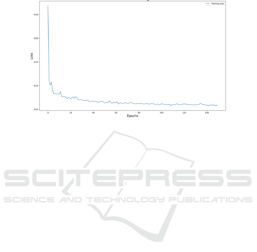
Figure 1: Traning loss for the LSTM RNN using Apple’s data (Photo/Picture credit: Original).

This article's Black Litterman model used the

basic structure of the traditional model while adding

a transformation process to consider the LSTM

prediction for determining the Ω matrix. This article's

LSTM(1d) model requires some assumptions of the

Black Litterman model to work correctly. Each

investor’s view consists of multiple expectations

about the assets. The mean value of those

expectations is expressed in the form of an investor’s

view in a q vector. The uncertainty of any view is the

variance of its set of expectations. For the single

LSTM Recurrent Neural Network to work properly,

investors in this article only give absolute views

(expectations) on assets. Further explanation is

provided to clarify how assumption one works. It

assumes investors make several expectations about

the future trend of the price of assets, and to represent

those expectations in view form, it takes the mean

value of expectations made on every single asset.

The transformation process is for the Black

Litterman model, which considers LSTM projection

data to adjust investors’investor's views. The

essential idea of the transformation process is to

adjust investors' views according to the LSTM

projection by adding LSTM projection data into the

expectation sets of views to change the mean value of

expectation sets. Adding LSTM projection data to the

expectation set will increase or decrease the view's

value (mean value of expectations), depending on

whether the investor has overvalued or undervalued

the stock performance compared to the LSTM model.

The amount of LSTM projected data added is

determined by the coefficient 𝜃. 𝜃 represents the ratio

of the number of LSTM data over the number of

original investors' expectations. The expression is

shown by:

𝑛



= 𝜃𝑛



(9)

Here, 𝜃 enables investors to choose the level they

believe in the LSTM model; this will be helpful in a

market revolution, which makes historical data fail to

predict future situations; when the market is in a

different situation, investors could choose the value

of 𝜃 to adapt to the market change. After the investor

gives the input of their original views on different

assets and chooses a value of 𝜃, the LSTM data will

be added to the expectation set according to the value

of 𝜃. The model calculates the new mean value of

expectation sets and generates a new Ω matrix. The

posterior return will be calculated based on the new

Ω matrix and new investor’s views, and the Black

Litterman model will take the value of the posterior

return to maximize the Sharpe ratio and generate the

final portfolio weight.

3 RESULTS AND DISCUSSION

3.1 Benchmark Portfolio

A benchmark portfolio is required for the exhibit

purpose to illustrate the result of the ML Black

Litterman model discussed in part 2. In the latter part,

the benchmark portfolio will be used as the stock

collection to let the model process it and generate an

adjusted final portfolio weight. The stock collection

(benchmark portfolio) is shown in the Table 1.

Investor’s View Adjustment of Black Litterman Model Based on LSTM Recurrent Neural Network

527

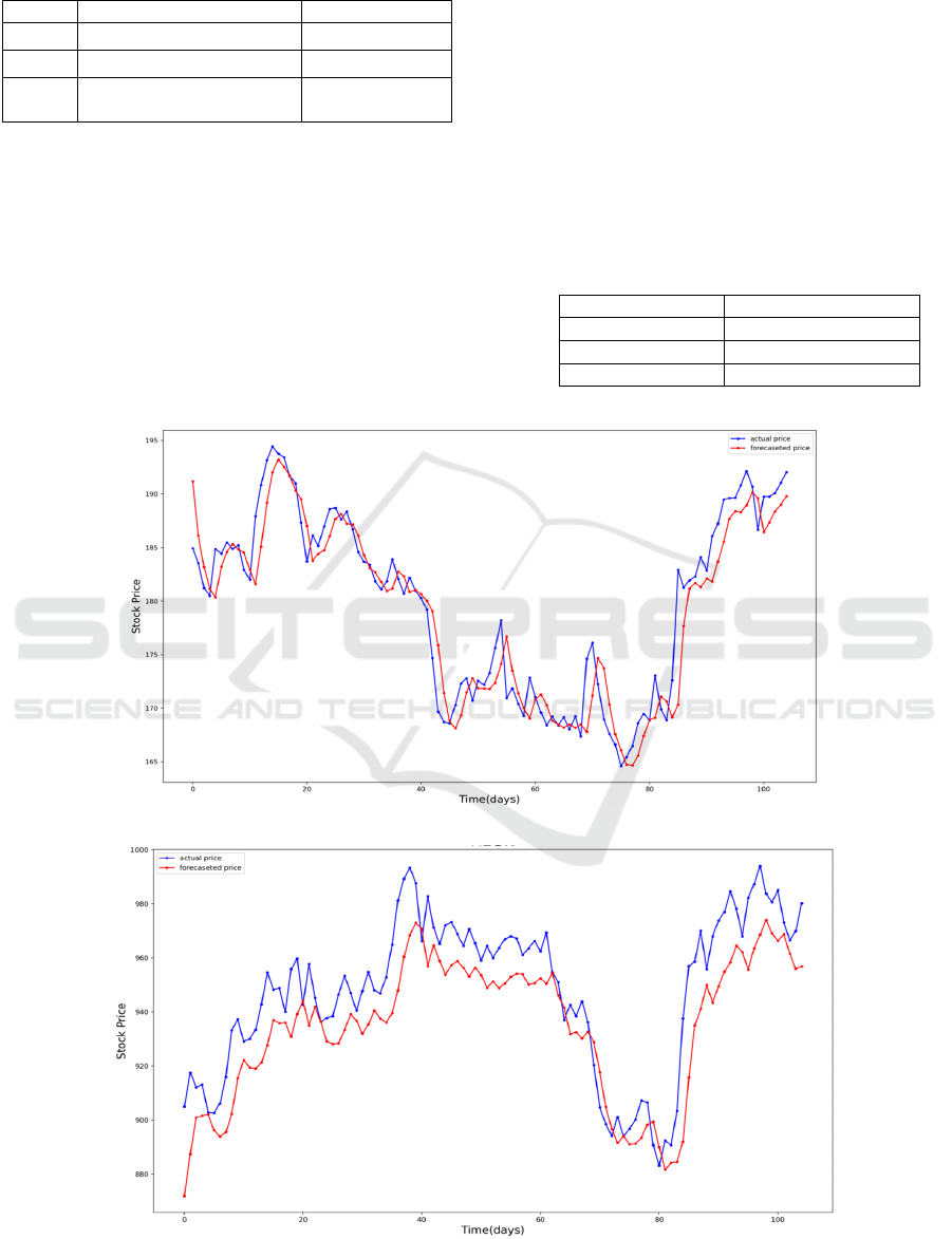
Table 1: Benchmark stock selection.

CODE Company Name Industry

AAPL Apple Inc. Smart Hardware

REGN Regeneron Pharmaceuticals Biotechnology

GE General Electricity

Aeros

ace

Manufacturing

3.2 LSTM Prediction Result

The LSTM is trained separately for different stocks

using the stock price data training set, which contains

more than 500 pairs of data representing the stock

data of the historical trading days. The training set

data takes the stock price from 2022-01-01 to 2024-

01-01; the test set is the stock price from 2024-01-01

to 2024-06-01. The result of the test for the

benchmark portfolio is shown below. Notice that the

virtual investor gives a view and expectations based

on the time point of 2024/8/8, and all data used to

build the Black Litterman model is collected at time

2024/8/8; this part only shows the general accuracy

of the model on selected stocks. Seen from Fig. 2, Fig.

3 and Fig. 4, the LSTM prediction data lags and the

price is over or under-projected. However, it is

enough to show the general market trend. The LSTM

projection result for each selected stock is shown in

the Table 2. The model is trained using the training

set of 2022/8/8 to 2024/8/8 and projects the stock

price data for the next trading day from 2024/8/8.

Table 2: LSTM projection results.

CODE LSTM projection

AAPL + 0.428%

REGN + 0.630%

TSLA + 0.179%

Figure 2: LSTM test result for AAPL (Photo/Picture credit: Original).

Figure 3: LSTM test result for REGN (Photo/Picture credit: Original).

ECAI 2024 - International Conference on E-commerce and Artiﬁcial Intelligence

528

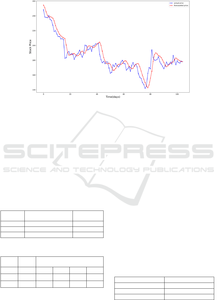
Figure 4: LSTM test result for TSLA (Photo/Picture credit: Original).

3.3 Black Litterman Model Build-up

Based on the Benchmark Portfolio

As mentioned in previous content, the posterior return

required a prior return, which is the market

equilibrium return illustrated by the market

capitalization (market portfolio weight). The price of

risk A is calculated using the indicator S&P500 index

to represent the market. After gathering the risk A

price, the market equilibrium return for each stock in

the benchmark portfolio can be calculated, as shown

in the Table 3. The market capitalization and other

data are collected for publishing earlier than 2024/1/1,

which stands from the perspective of the virtual

investor. The expectation sets are shown in Table 4.

Table 3: Prior returns for benchmark portfolio.

CODE Market Cap

(Trillion USD)

Prior Return

AAPL 3.23 0.14%

REGN 0.115 0.03%

TSLA 0.631 0.22%

Table 4: Expectation sets for views on the benchmark

portfolio.

CODE View

(

mean

)

Expectations

AAPL 0.44% 0.50% 0.35% 0.47% 0.43%

REGN 0.66% 0.53% 0.74% 0.58% 0.78%

TSLA 0.53% 0.45% 0.49% 0.56% 0.61%

The prior return rate must be adjusted through the

Bayesian law to get the posterior return. This process

requires the investor’s view and LSTM projection as

coefficient 𝜃. The investor’s view is expressed

through the q vector and matrix p. For exhibit

purposes, investors will give an impractical view

(multiple expectations) of Tesla’s stock. The

expectation sets for views are shown following the q

vector and p matrix.

𝑞= 

0.44%

0.66%

0.53%

; 𝑝= 

100

010

001



(9)

Without any LSTM projection being added, the

expectation set of views will be equal to the table

provided above. In this situation, the Ω matrix for

original expectation sets is shown below, which

simply takes the variance of each expectation set for

its diagonal elements.

Ω= 

0.00000043 0 0

0 0.0000015 0

0 0 0.00000051



(10)

The posterior return could be calculated using the

Bayesian method mentioned in the previous part. For

the case without LSTM adjustment, the posterior

return is shown in the Table 5. Based on the posterior

return shown, the final portfolio weight can be

calculated to maximize the Sharpe ratio, as shown in

the Table 6.

Table 5: Posterior returns for benchmark portfolio.

CODE Posterior return

AAPL 0.43%

REGN 0.65%

TSLA 0.53%

Investor’s View Adjustment of Black Litterman Model Based on LSTM Recurrent Neural Network

529

Table 6: Portfolio weight generated for the benchmark portfolio and other information.

AAPL REGN TSLA

Weight 32.31% 65.53% 2.16%

Posterior return 0.43% 0.65% 0.53%

Sharpe ratio 0.425

Sum of weight 100%

Expected return 0.00581

Standard Deviation 0.0133

Risk free interest rate 4%

Table 7: Expectation sets for views on the benchmark portfolio (with LSTM).

Code View (mean) Expectations LSTMs

AAPL 0.43% 0.50% 0.35% 0.47% 0.43% 0.43% 0.43% 0.43%

REGN 0.65% 0.53% 0.74% 0.58% 0.78% 0.63% 0.63% 0.63%

TSLA 0.38% 0.45% 0.49% 0.56% 0.61% 0.18% 0.18% 0.18%

However, this portfolio failed to consider the

actual market situation. As previously mentioned, the

LSTM projected data needs to be added to solve this

problem. In this case, assume the investor set 𝜃

equals 0.75, indicate there will be three identical

LSTM projected data added to the expectation set,

and show the expectation set that has been adjusted in

Table 7. It is clear to see that the view on Tesla

becomes smaller and closer to the market trend,

which is illustrated by the LSTM model. The q vector

and p matrix could be generated through this table

above in a similar way to the previous case without

LSTM adjustment. The q vector, p matrix, and Ω

matrix are shown as:

𝑞= 

0.43%

0.65%

0.38%

; 𝑝= 

100

010

001



(11)

Ω= 

0.00000022 0 0

0 0.00000076 0

0 0 0.0000037



(12)

The posterior return thus, can be calculated using q

vector, p matrix, and Ω matrix. The resturns are

shown in Table 8. With the adjusted posterior return

provided, the final portfolio weight could be

calculated according to the rule to maximize the

Sharpe ratio, shown in the Table 9.

Table 8: Posterior returns for the benchmark portfolio (with

LSTM).

CODE Posterior return

AAPL 0.43%

REGN 0.64%

TSLA 0.38%

Table 9: Portfolio weight generated for the benchmark

portfolio and other information (with LSTM).

AAPL REGN TSLA

Wei

ht 34.84% 65.16% 0.00%

Posterior return 0.43% 0.64% 0.38%

Sharpe ratio 0.420

Sum of weight 100%

ected return 0.00570

Standard

Deviation

0.0132

Risk free interest

rate

There is a significant difference in Tesla's weight

in the LSTM adjusted and unadjusted portfolio; the

difference will be illustrated and explained in the

following parts.

3.4 Comparisons

According to the result portfolio generated in part 3.2.

The portfolio generated without the LSTM

adjustment invests 2.16% of Tesla's assets, while the

portfolio generated without the LSTM adjustment

decides not to invest in Tesla. The difference between

portfolios generated is due to the difference in Tesla's

posterior return. Without the LSTM adjustment, the

posterior return trend strictly follows the original

investor's view; in the abovementioned case, the

investor gives an impractical (bold) view of Tesla

with an expected return mean value of 0.53%.

Without LSTM adjustment, the posterior return

calculated for Tesla will be estimated at 0.53%,

almost identical to the investor's view because of the

relatively low variance (uncertainty) of view on Tesla.

However, the market trend illustrated by the LSTM

has a value of 0.179%. When the case investor's view

differs from the LSTM result, investors could choose

ECAI 2024 - International Conference on E-commerce and Artiﬁcial Intelligence

530

to use LSTM adjustment. In the previous case, the

investor chose to use an LSTM adjustment with 𝜃

equal to 0.75; after the adjustment, the posterior

return became 0.38%, closer to the market trend. The

uncertainty of view is reconsidered, and the variance

of each view has also been re-calculated. Tesla has a

higher weight in the case without LSTM adjustment

because of its higher posterior return. In the case of

LSTM adjustment, the posterior return decreased;

thus, to maximize the Sharpe ratio, the risk of Tesla

will not be worth investing in for its lower posterior

return.

3.5 Limitations and Prospects

The model could provide a direction for research to

explore more advanced asset management methods.

However, it has some limitations that could hinder

implementing the model in the real market. The

LSTM(1d) model limits the time one view handles; in

practice, investors often give a view for the asset

value in future months or even years; the LSTM(1d)

model limits investors to give views only for

tomorrow. The accuracy of the LSTM model in

illustrating price fluctuation is good, but it is lagged;

thus, when the price trend appears as a turning point,

the LSTM model may give an opposite result

compared to the actual future trend. The single LSTM

model used in the Black Litterman model limited

investors from being able to give relative views on

assets because it requires a comparison between

LSTM results. Those limitations could be solved by

improving the LSTM model to make it more accurate

and time-catching.

4 CONCLUSIONS

To sum up, the research explored combining the

LSTM Recurrent Neural Network and Black

Litterman model, integrating machine learning

methods and asset management. The study

demonstrates that the method LSTM projections can

adjust investor views, enabling a more market-

aligned portfolio allocation by comparing the

portfolio weight generated through the ML method

and the non-ML method for the benchmark portfolio.

The training process design and loss result control for

the LSTM model ensured accuracy when using

LSTM projections to simulate and forecast the market

trend. Further research is necessary to improve the

limitations of the model discussed in this research;

improving the projection period and accuracy of the

LSTM Recurrent Neural Network and practicing

another method to combine machine learning and

portfolio management models may contribute to the

market meaning of the model discussed. By

incorporating machine learning forecasts, this

enhanced model offers investors a flexible approach

that adjusts to market trends when their views diverge

significantly from the market, and this would be

helpful for new-entrance investors. The result

analysis of the model meanwhile proved the

effectiveness of using a time series machine learning

algorithm to control the investor’s view input term

REFERENCES

Barua, R., Sharma, A. K., 2022. Dynamic Black Litterman

portfolios with views derived via CNN-BiLSTM

predictions. Finance Research Letters, 49, 103111.

Barua, R., Sharma, A. K., 2023. Using fear, greed and

machine learning for optimizing global portfolios: A

Black-Litterman approach. Finance Research Letters,

58, 104515.

Black, F., Litterman, R., 1992. Global portfolio

optimization. Financial analysts journal, 48(5), 28-43.

Fabozzi, F. J., 2012. Encyclopedia of Financial Models.

Wiley eBooks.

Hampus, E., 2021 The Black-Litterman Asset Allocation

Model: An Empirical Analysis of Its Practical Use.

Master desertation of KTH Royal Institute of

Technology

He, G., Litterman, R., 2002. The intuition behind Black-

Litterman model portfolios. Available at SSRN: 334304.

Li, C., Chen, Y., Yang, X., Wang, Z., Lu, Z., Chi, X., 2022.

Intelligent black–Litterman portfolio optimization

using a decomposition-based multi-objective DIRECT

algorithm. Applied Sciences, 12(14), 7089.

Mankert, C., 2006. The BlackLitterman Model. PhD thesis.

KTH Royal Institute of Technology.

Markowitz, H., 1952. Modern portfolio theory. Journal of

Finance, 7(11), 77-91.

Min, L., Dong, J., Liu, D., Kong, X., 2021. A black-

litterman portfolio selection model with investor

opinions generating from machine learning algorithms.

Engineering Letters, 29(2), 710-721.

Satchell, S., Scowcroft, A., 2007. A demystification of the

Black-Litterman model: Managing quantitative and

traditional portfolio construction. Forecasting expected

returns in the financial markets, 39-53.

Sun, R., Stefanidis, A., Jiang, Z., Su, J., 2024. Combining

Transformer based Deep Reinforcement Learning with

Black-Litterman Model for Portfolio Optimization.

arXiv preprint arXiv:2402.16609.

van de Schoot, R., Depaoli, S., King, R., et al., 2021.

Bayesian statistics and modelling. Nature Reviews

Methods Primers, 1(1), 1.

Investor’s View Adjustment of Black Litterman Model Based on LSTM Recurrent Neural Network

531