Comparative Analysis of Random Forest and LSTM Models in

Predicting Financial Indices: A Case Study of S&P 500 and CSI 300

Yuxuan Qian

School of Mathematics, The University of Edinburgh, Edinburgh, U.K.

Keywords: Stock Market Prediction, Machine Learning, Random Forest, Long Short-Term Memory Network, Sliding

Window.

Abstract: Stock market prediction has long been a topic of significant interest due to its potential financial rewards and

the inherent complexity of financial markets. This study investigates the application of two machine learning

models, Random Forest (RF) and Long Short-Term Memory networks (LSTM), in predicting the closing

prices of the Standard & Pooler’s 500 Index (S&P 500) and the Shanghai Shenzhen 300 Index (CSI 300)

indices using historical data from 09/08/2021 to 08/08/2024 by various indicators, respectively. A sliding

window method was used to make predictions based on historical data points. The evaluation metrics

including R2, Mean Absolute Error (MAE), and Root Mean Squared Error (RMSE) were used to assess the

models' performance. According to the data, LSTM outperforms RF in CSI 300 prediction while RF performs

better in S&P 500 prediction. This study shows the applicability of various models and offers empirical

support for optimizing asset price prediction models.

1 INTRODUCTION

The Efficient Market Hypothesis (EMH), proposed

by Fama (1970), suggests that stock prices fully

reflect all available information and follow a random

walk, implying that future price movements are

unpredictable (Fama, 1970). However, critics of

EMH argue that there are inefficiencies in the market

that can be exploited using advanced analytical

techniques, such as machine learning (Daniel,

Hirshleifer & Subrahmanyam, 1998; Bondt & Thaler,

1990).

In recent years, numerous studies have explored

the application of various methods in stock price

prediction, including classifier ensembles (Basak,

Kar, Saha, Khaidem, & Dey, 2019; Lohrmann &

Luukka, 2019; Singh & Malhotra, 2023), support

vector machines (Sedighi, Jahangirnia, Gharakhani,

& Fard, 2019), neural networks (Baek & Kim, 2018;

Das, Sadhukhan, Chatterjee, & Chakrabarti, 2024),

and deep learning (Dang, Sadeghi-Niaraki, Huynh,

Min, & Moon, 2018; Patil, Parasar, & Charhate,

2023; Rath, Das, & Pattanayak, 2024). These studies

provide multiple technical approaches to improve

prediction accuracy. Ensemble methods like Random

https://orcid.org/0009-0008-0698-5353

Forest and deep learning models like Long Short-

Term Memory Networks (LSTM) have shown

promise in this domain (Kumbure M. M., Lohrmann,

Luukka, & Porras, 2022). Given the evolving and

complex nature of market environments, especially in

the United States and China, significant challenges

remain in stock price forecasting.

Thus, this study predicts the closing price of two

leading market indices (S&P 500 and CSI 300) by RF

and LSTM among different predictors (Close price,

10,50,100-days Moving Averages, Daily Change,

and Log Difference) using a sliding window

approach. This technique involves using a fixed

window of previous data points (in this case, 1, 60,

120, 240, 360, and 480 days) to predict the next day

closing price. The results demonstrate that the

effectiveness of prediction models is closely tied to

the characteristics of the financial market being

analyzed. While RF proves to be more consistent and

effective for the S&P 500, particularly with smaller

window sizes, LSTM shows its strength in capturing

long-term dependencies, making it more suitable for

predicting the CSI 300 with moderate window sizes.

These insights underscore the importance of carefully

selecting both the model and the window size based

Qian, Y.

Comparative Analysis of Random Forest and LSTM Models in Predicting Financial Indices: A Case Study of S&P 500 and CSI 300.

DOI: 10.5220/0013268700004568

In Proceedings of the 1st International Conference on E-commerce and Artiﬁcial Intelligence (ECAI 2024), pages 453-461

ISBN: 978-989-758-726-9

453

on the unique attributes of the data and the objectives

of the analysis.

2 DATA

2.1 Dataset

The datasets of the S&P 500 and the CSI 300 Index

come from the Yahoo Finance website, which

captures the daily High, Low, Close price, and

Volume of each index from 09/08/2021 to

09/08/2024.

Table 1 and Table 2 show the basic information

of the datasets with an additional 5 columns MA10,

MA50, MA100, Daily Change, and Log Diff that

were added manually.

The S&P 500’s combination of lower Close

standard error (std) but higher mean Close price and

higher Daily Change std suggests a market that is

generally stable in the long run but more reactive and

possibly more liquid daily. In contrast, the CSI 300

might reflect a market with more significant long-

term uncertainty but less short-term sensitivity.

Meanwhile, the average daily change for the S&P 500

is positive, meaning that the overall price for this

index is appreciating, while the CSI 300 is

depreciating.

The moving average (MA) establishes a

continuously updated average price to smooth out

price data. It reduces noise on a price chart and

provides information about the overall direction of

prices. The amount of lag is determined by the

moving average period selected; longer durations

result in more lag. Investors and traders often follow

the 10-, 50- and 100-day moving averages as

significant trading signals. As shown in Figure 1, the

best value to measure the MA is between 10 and 50

days because it still captures trends in the data without

noise.

Log Difference is a logarithmic transformation of

the ratio of consecutive closing prices. It is calculated

as: 𝐿𝑜𝑔𝐷𝑖𝑓𝑓𝑒𝑟𝑒𝑛𝑐𝑒 = 𝑙𝑜𝑔

Close Price

today

Close Price

yesterday

 . It is

often used to stabilize variance and to make the time

series more stationary. In financial time series, prices

tend to exhibit heteroskedasticity (Nelson & Daniel,

1991), meaning the variance of the returns can change

over time. By taking the log difference, the models

can better capture the relative price movements in a

way that is less influenced by large, erratic price

jumps.

Table 1: S&P500 Overview.

High Low Close Volume MA10 MA50 MA100 Log Diff

Count 755 755 755 755 746 706 666 754

Mean 4465.80256 4411.63341 4439.88951 4.20392e+09 4434.64056 4403.96094 4373.04579 0.00024

Std 465.89983 473.36562 469.50128 8.49080e+08 463.73393 425.87432 392.43195 0.01104

Min 3608.34009 3491.58008 3577.03003 1.63950e+09 3642.97698 3787.07001 3850.07701 -0.04420

25% 4114.92505 4061.65002 4090.39499 3.72544e+09 4067.82249 4025.43906 4016.92924 -0.00602

50% 4422.62012 4371.97022 4398.95020 4.49526e+09 4400.65544 4393.39830 4385.53238 0.00041

75% 4706.50513 4661.23999 4686.00000 4.02095e+09 4666.10402 4611.87985 4565.25610 0.006838

Max 5669.66992 5639.02002 5667.20020 9.35428e+09 5598.21006 5449.65120 5320.81369 0.05395

Table 2: CSI 300 Overview.

High Low Close Volume MA10 MA50 MA100 Log Diff

Count 728 728 728 728 719 679 639 727

Mean 4037.96092 3985.41449 4012.18025 1.3354+e09 4010.22511 4000.76741 3986.66531 -0.00055

Std 486.18919 479.72145 483.21358 36499.76036 474.73090 443.35882 396.40565 0.01024

Min 3233.85010 3108.35010 3179.62988 64800.00000 3254.78899 3325.35061 3429.25860 -0.05068

25% 3633.92743 3601.185056 3615.13245 107700.00000 3619.50148 3618.68899 3682.73260 -0.00678

50% 3976.05994 3927.41003 3953.83496 127900.00000 3945.06694 3949.38198 3947.04989 -0.00112

75% 4261.972657 4191.29504 4225.83997 152025.00000 4215.83750 4197.76730 4167.85590 0.00558

Max 5143.83984 5079.72998 5083.799801 326700.00000 5007.33501 4913.34303 4905.59002 0.04234

ECAI 2024 - International Conference on E-commerce and Artiﬁcial Intelligence

454

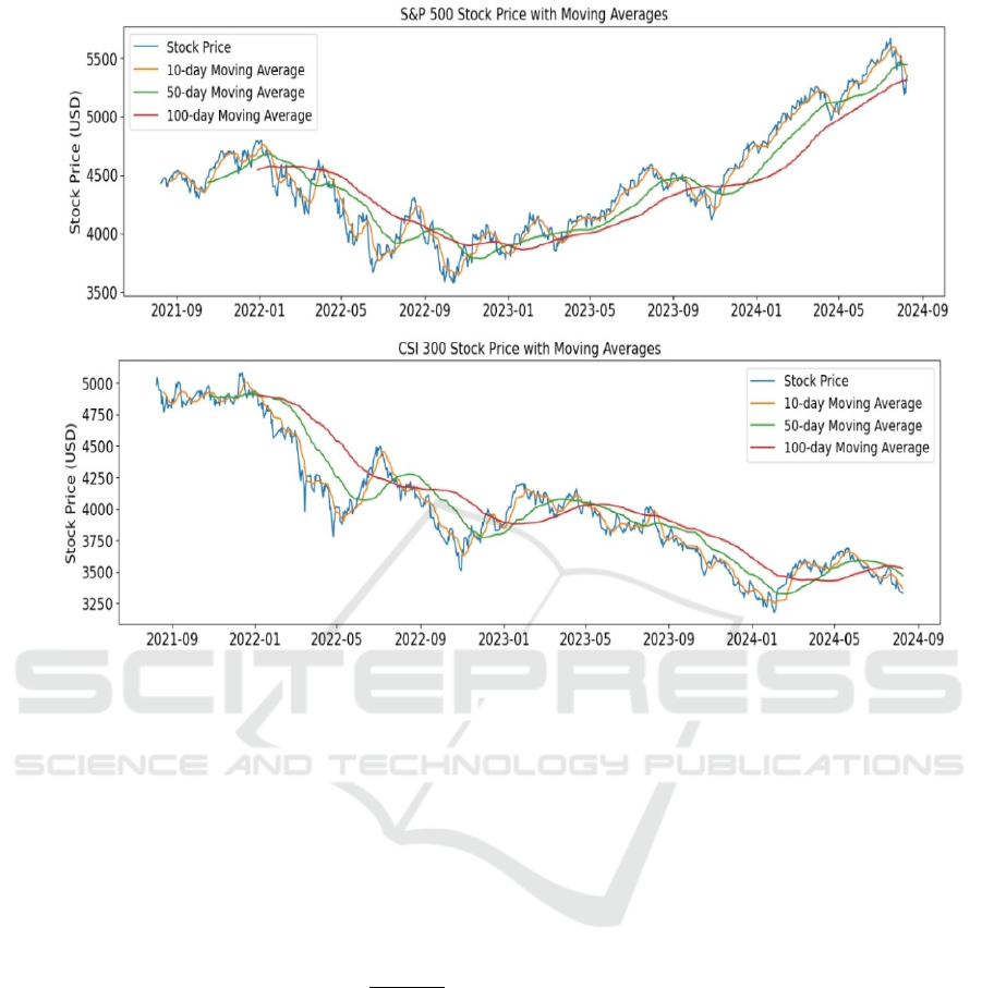
Figure 1: S&P 500 visualization with different MA (above), CSI 300 visualization with different MA (below).

2.2 Data Preprocessing

Normalization is an important preprocessing step in

machine learning, especially for LSTM that is

sensitive to the scale of input feature (Patro & Sahu,

2015). It ensures that all features make an equal

contribution to the model training process. Min-Max

Scaler is a simple and effective data normalization

technique that preserves the relationships between the

original data points. The scaling is performed

according to the formula: 𝑋





min



max



min

𝑤ℎ𝑒𝑟𝑒 𝑋 is the original feature value, and the

minimum and maximum values of the feature in the

dataset are represented by 𝑋

min

and 𝑋

max

. By applying

this transformation, the values of each characteristic

are mapped to 0 and 1, respectively.

3 METHODOLOGIES

3.1 Random Forest

The foundation of Random Forest is to create many

decision trees during training and produce the average

forecast of each tree separately. The model's

robustness and predictive performance are enhanced

by this ensemble technique (Breiman, 2001). Figure

2below is a flow map for RF.

Randomness is introduced in two keyways.

Firstly, Bootstrap Aggregating (1): For each tree, a

subset of the training data is chosen. This step ensures

that every tree is trained on different subsets of data,

adding variability and reducing overfitting. Secondly,

Feature Randomness (2): A random subset of features

is taken into consideration for splitting at each

decision tree node. Finally averages the n predictions

made by individual trees.

Grid Search is a popular tuning parameter

technique that improves model performance. It works

through multiple combinations of hyperparameter

values from giving parameter space. It is effective

when the parameter space is manageable, and thus

can be applied to RF. The GridSearchCV from Scikit-

learn uses cross-validation, which reduces

overfitting.

Comparative Analysis of Random Forest and LSTM Models in Predicting Financial Indices: A Case Study of S&P 500 and CSI 300

455

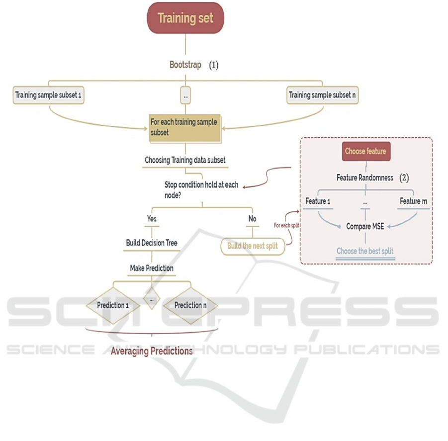
Figure 2: Flow map for Random Forest Regression

3.2 Long Short-Term Memory

Network (LSTM)

LSTM is a deep learning method used to identify

long-term dependencies in sequential data

(Hochreiter & Schmidhuber, 1997). It is ideally suited

for time series forecasting, which includes stock price

prediction because it makes use of memory cells to

store information over time. The forget gate, input

gate, and output gate are components of the

architecture of the LSTM model (Hochreiter &

Schmidhuber, 1997).

Key formulas for LSTM are:

Forget Gate 𝑓



: selects which data from the cell

state should be discarded. Takes 𝑥



and ℎ



inputs, processes them through weight matrices and

bias, and then applies sigmoid activation.

𝑓



= 𝜎𝑊



⋅



ℎ



, 𝑥





𝐵





(1)

Input Gate 𝑖



: Selects the new data to be stored in

the cell state.

𝑖



= 𝜎



𝑊



⋅



ℎ



, 𝑥





𝐵





(2)

Cell State Update 𝑐



.: Uses the sigmoid function

to regulate information and filters values using the

inputs ℎ



and 𝑥



. The tanh function is used to

generate a vector.

𝑐



𝑓



⋅𝑐



𝑖



⋅𝑡𝑎𝑛ℎ



𝑊



⋅



ℎ



, 𝑥





𝐵





(3)

Output Gate 𝑜



: Selects the appropriate output in

accordance with the cell state. Sigmoid function to

regulate information.

𝑜



= 𝜎



𝑊



⋅



ℎ



, 𝑥





𝑏





(4)

Where: ℎ



= 𝑜



⋅𝑡𝑎𝑛ℎ



𝑐





is the hidden state 𝑥



is the input at time step 𝑡. 𝑊



, 𝑊



, 𝑊



, 𝑊



are weight

matrices. 𝐵



, 𝐵



, 𝐵



, 𝐵



are bias terms. 𝜎 is the

sigmoid function.

These gates enable LSTMs to selectively retain

important information over extended periods, making

them effective for processing and predicting

sequential data (Lin, Tino, & Giles, 1996).

ECAI 2024 - International Conference on E-commerce and Artiﬁcial Intelligence

456

4 RESULTS

Apply each model to 6 predictors (Close Price,

MA10, MA50, MA100, Daily Change, Log

Difference) individually across 6 different window

sizes (1, 60, 120, 240, 360, 480) for two indexes (S&P

500 and CSI 300). So, for each model, 72 estimations

are obtained, and evaluated by RMSE, MAE, and R2.

4.1 Random Forest

Table 3 shows the ratio between the evaluation

metrics of the model with the best parameter found by

GridSearchCV and the model with default value.

The average performance for RMSE and MAE

reduced by around 75% to 94%, which means the

model does improve pretty much. Then table 4

displays the information on evaluation metrics

applying the RF model.

With a mean R2 value of 0.9869, the model can

account for approximately 98.69% of the variation

observed in the target variable. This is an excellent

result that demonstrates how well the model explains

the variance in the data. Meanwhile, the std is very

low (0.0185), and the minimum R2 value (0.8864),

indicates consistent performance across different

predictors and window sizes.

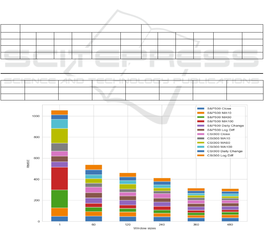
RMSE penalizes larger errors more than MAE,

making it susceptible to outliers. The mean RMSE is

42.95, which is higher than the MAE, suggesting that

the model may struggle with outliers. Let’s further

analyze the large variance in RMSE graphically.

As showing in Figure, increasing the window size

results in a decrease in RMSE, indicating that using

more historical data leads to better predictions.

However, the gradient for such diminishing is slower

for window sizes larger than 360, and large window

sizes are computationally exhaustive, hence 360 is a

preferable window size.

Table 3: Improvements after Grid Search.

S&P 500 CSI 300

Close MA10 MA50 MA100 Daily Change Log Diff Close MA10 MA50 MA100 Daily Change Log Diff

RMSE 0.941 0.791 0.797 0.805 0.942 0.838 0.845 0.763 0.792 0.881 0.825 0.877

MAE 0.936 0.838 0.830 0.841 0.882 0.821 0.862 0.754 0.839 0.946 0.813 0.903

R2 1.001 1.009 1.048 1.075 1.001 1.003 1.002 1.013 1.044 1.009 1.006 1.002

Table 4: Evaluation Metric for Random Forest.

mean std min 25% 50% 75% max

0.986987 0.018553 0.886376 0.99003 0.993367 0.995382 0.998121

RMSE 42.951008 31.303382 18.878831 28.464084 35.197097 46.129500 214.560327

MAE 32.053035 21.676995 15.001533 21.865735 27.430513 32.413918 145.967554

Figure 3: Total RMSE for RF across different window sizes.

Comparative Analysis of Random Forest and LSTM Models in Predicting Financial Indices: A Case Study of S&P 500 and CSI 300

457

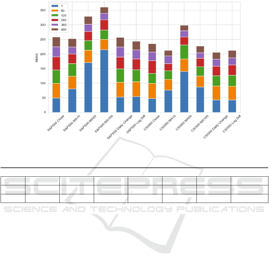
Figure 4: Total RMSE for RF across different predictors.

Table 5:

Evaluation Metric for LSTM

mean std min 25% 50% 75% max

0.818179 0.140656 0.335637 0.773241 0.873154 0.913501 0.960913

RMSE 45.817748 22.295338 11.849076 29.754566 40.982957 50.408349 132.253446

MAE 37.133658 20.818579 10.880780 23.272937 30.825190 43.859155 123.335092

Figure 4 shows that the predictors MAs appear to be

less effective for smaller window sizes. Still, for

larger window sizes, the Close RMSE is quite small,

which is only half of the mean value. Other indicators

like Close Price, Daily Change, and Log Diff have

more consistent performance across different window

sizes but are still improved.

The S&P 500 and the CSI 300 indices show

similar trends in RMSE across different indicators

and window sizes, suggesting that the model's

behavior is consistent.

4.2 Long Short-Term Memory

Similarly, the evaluation metrics for LSTM are

presented as below in Table 5.

On average, the LSTM model explains

approximately 81.82% of the variance in the target

variable, which is a good predictive capability. The

variance in R² (0.141) and the minimum R² (0.336)

suggests that the model is poor in some cases.

However, the interquartile Range (IQR), 0.773 to

0.914, indicates that the model performs quite well in

most cases.

The gap in RMSE and MA suggests that there

might be some outliers, leading to occasional large

errors. Noticeably, the high values in the std of RMSE

and MAE suggest that the error magnitude varies

considerably across different predictions, thus more

exploration based on RMSE is done (Figure 5).

From Figure 5, there is an initial decrease in

RMSE as the model has access to more historical

data. For window sizes 60 to 120, the RMSE

stabilizes with minor fluctuations, suggesting that

additional historical data does not necessarily lead to

substantial improvements in predictions. There is a

slight increase in RMSE as the window size extends

beyond 240 days. This could indicate that the model

is starting to overfit the training data as the window

size increases. From Figure 6, RMSE for MA10 and

MA50 is generally lower compared to other

predictors, which is consistent with the conjecture by

Figure 1, that the best value for MA is between 10 and

50 days. Still, Daily Change, and Log Difference have

a consistent performance across different window

sizes.

ECAI 2024 - International Conference on E-commerce and Artiﬁcial Intelligence

458

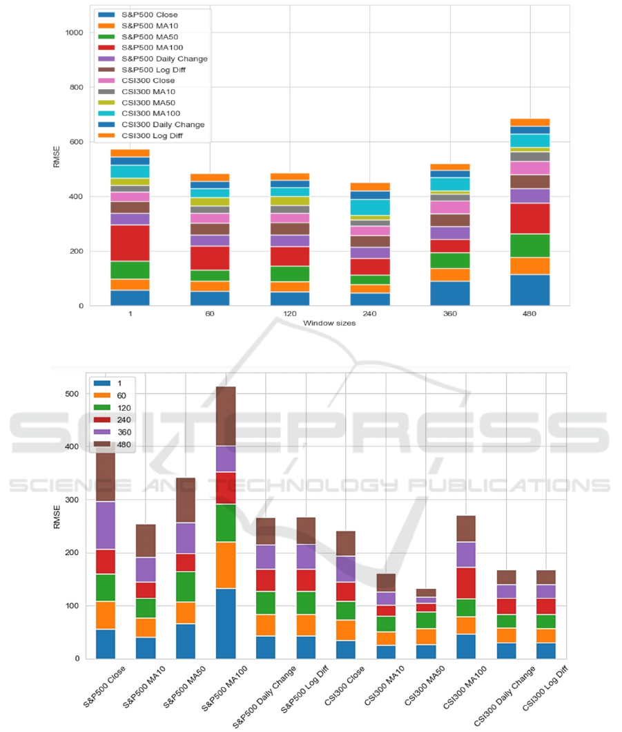
Figure 5: Total RMSE for LSTM across different window sizes.

Figure 6: Total RMSE for LSTM across different predictors

The model's performance is generally better on the

CSI 300 index compared with the S&P 500,

indicating potential market-specific differences that

could be due to the model's sensitivity to certain

market conditions (analysis by Table 1 and Table 2)

4.3 Comparison Between RF and

LSTM

In the above section, the model performance is

analyzed individually. It is also important to compare

the two models together to make further conclusions.

Comparative Analysis of Random Forest and LSTM Models in Predicting Financial Indices: A Case Study of S&P 500 and CSI 300

459

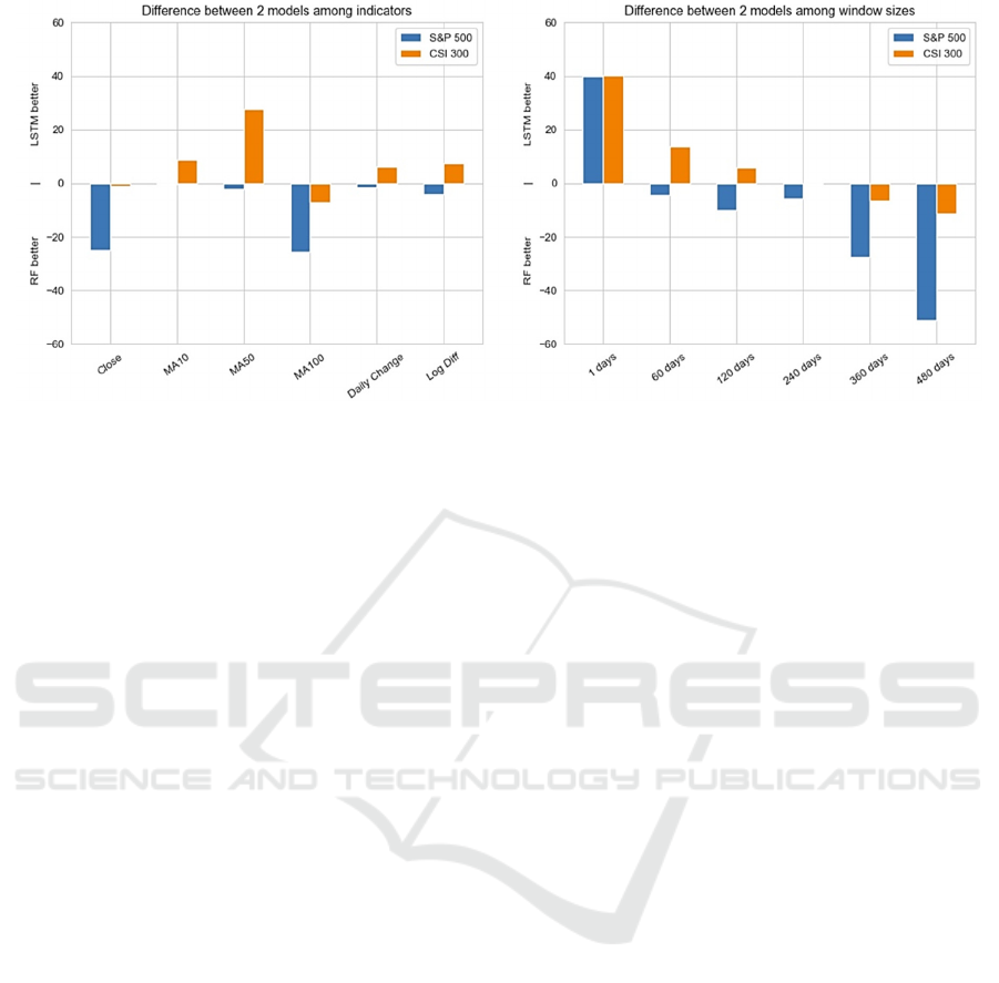
Figure 7: Comparison between RF and LSTM among different predictors (left), Comparison between RF and LSTM among

different window sizes (right).

From Table 4 and table 5 the LSTM tends to have a

higher mean and IQR prediction errors, but it also has

the potential to make more precise predictions in its

best cases, the lowest RMSE is 11.849. This suggests

that LSTM outperforms RF in its best scenarios. On

the other hand, RF with a lower mean and a narrower

IQR of RMSE shows a more consistent performance.

From Figure 7 (left), LSTM shows strengths in

handling indicators like MA10 and MA500, while RF

generally performs better with indicators like Close

and M100. The performance differences between the

two models vary depending on the index, suggesting

that model effectiveness might be market specific.

For the S&P 500, RF is generally better among all

predictors, while LSTM is better for the CSI 300.

From Figure 7 (right), LSTM excels in very short-

term predictions, due to high RMSE in RF predicted

by window size 1 (Figure 3). For median window

sizes (60-240 days), the different performance among

the two models depends on the index, in specific, RF

is better for the S&P 500 and the LSTM is better for

CSI 300, which is similar to different indicators as

above. For extreme long-term predictions, RF gains

an advantage as the window size increases.

5 CONCLUSIONS

This paper explored the application of RF and LSTM

models in predicting the closing prices of the S&P

500 and CSI 300 indices using various financial

indicators. The performance of these models is

contingent on the characteristics of the specific

dataset being analyzed. For the S&P 500 index, RF

consistently outperforms LSTM, particularly for

small window sizes. This suggests that RF's ability to

capture complex interactions between features

without relying on sequential dependencies makes it

better suited for the S&P 500. On the other hand,

LSTM excels in predicting the CSI 300 index for

moderate window sizes which is more

computationally efficient than large window sizes.

This indicates the CSI 300 benefit from LSTM’s

strength in capturing long-term dependencies in time

series data。 Also, the choice between LSTM and RF

should be guided by the specific needs of the

prediction task. If avoiding large errors is crucial,

LSTM may be preferable. However, if consistency is

prioritized, RF might be the better choice. Moreover,

increasing the window size does not always enhance

model performance. Moreover, the diminishing

returns observed for larger windows in the LSTM

suggest that the choice of window size should be

carefully tailored to the specific market and data

characteristics.

Hybrid approaches that combine different

machine learning models to increase prediction

accuracy may be investigated in future studies.

Additionally, incorporating more market data and

external factors, such as macroeconomic indicators

and international political events, could enhance the

models’ applicability and generalizability.

REFERENCES

Baek, Y., & Kim, H. Y. (2018). ModAugNet: A New

forecasting framework for stock market index value

with an overfitting prevention LSTM module and a

ECAI 2024 - International Conference on E-commerce and Artiﬁcial Intelligence

460

prediction LSTM module. Expert Systems With

Applications, 113(DEC.), 457-480.

Basak, S., Kar, S., Saha, S., Khaidem, L., & Dey, S. R.

(2019). Predicting the direction of stock market prices

using tree-based classifiers. North American Journal Of

Economics And Finance, 47, 552-567.

Bondt, W. D., & Thaler, R. (1990). Do security analysts

overreact? The American Economic Review, pp. 80,

52-57.

Breiman, L. (2001). Random forests, machine learning 45.

Journal of Clinical Microbiology, 2, 199-228.

Dang, L. M., Sadeghi-Niaraki, A., Huynh, H. D., Min, K.,

& Moon, H. (2018). Deep learning approach for short-

term stock trends prediction based on two-stream gated

recurrent unit network. IEEE Access, 6, 55392-55404.

Daniel, K., Hirshleifer, D., & Subrahmanyam, A. (1998).

Investor Psychology and Security Market Under and

Overreactions. The Journal of Finance, 53: 1839-1885.

Das, N., Sadhukhan, B., Chatterjee, R., & Chakrabarti, S.

(2024). Integrating sentiment analysis with graph

neural networks for enhanced stock prediction: a

comprehensive survey. Decision Analytics Journal, 10.

Fama, E. (1970). Efficient market hypothesis: A Review of

Theory and Empirical Work.

Hochreiter, S., & Schmidhuber, J. (1997). Long short-term

memory. Neural Computation, 9(8), 1735-1780.

Kumbure, M. M., Lohrmann, C., Luukka, P., & Porras, J.

(2022). Machine learning techniques and data for stock

market forecasting: A literature review. Expert Systems

with Applications, Volume 197, 2022, 116659, ISSN

0957-4174.

Lin, T., Tino, P., & Giles, C. L. (1996). Learning long-term

dependencies in NARX recurrent neural networks.

IEEE Transactions on Neural Networks, 7(6), 1329-

1338.

Lohrmann, C., & Luukka, P. (2019). Classification of

intraday s&p500 returns with a random forest.

International Journal of Forecasting, 35(1), 390-407.

Nelson, D. B. (1991). Conditional heteroskedasticity in

asset returns: a new approach. Modelling. Stock Market

Volatility, 59(2), 347-0.

Patil, P. R., Parasar, D., & Charhate, S. (2023). An effective

deep learning model with reduced error rate for accurate

forecast of stock market direction. Intelligent decision

technologies: An international journal, 17(3), 621-639.

Patro, S. G., & Sahu, K. K. (2015). Normalization: a

preprocessing stage.

Rath, S., Das, N. R., & Pattanayak, B. K. (2024). Stacked

BI-LSTM and E-optimized CNN-A hybrid deep

learning model for stock price prediction. Optical

Memory and Neural Networks.

Sedighi, M., Jahangirnia, H., Gharakhani, M., & Fard, S. F.

(2019). A novel hybrid model for stock price

forecasting based on metaheuristics and support vector

machine. 4(2), 75.

Singh, H., & Malhotra, M. (2023). A novel approach of

stock price direction and price prediction based on

investor's sentiments. SN Computer Science, 4(6), 1-

10.

Comparative Analysis of Random Forest and LSTM Models in Predicting Financial Indices: A Case Study of S&P 500 and CSI 300

461