Irregular Stock Data Prediction Performance Optimisation Based on

the Simple Linear Interpolation

Zhenyu Xu

Warwick Manufacturing Group, University of Warwick, Coventry, U.K.

Keywords: Machine Learning, Data Pre-Processing, Interpolation, Irregular Data.

Abstract: This study examines how Simple Linear Interpolation (SLI) affects stock data’s irregular data processing and

prediction performance of machine learning models. Using Tesla stock data over ten years, this study cleansed,

normalised, and applied SLI methods to reduce missing values and inconsistencies in the data. Then, the

performance of the models before and after interpolation was evaluated by constructing various machine

learning models, including XGBoost, Random Forest, K Nearest Neighbour (KNN) and Stacked Model. The

experimental results suggest that SLI enhance the models' performance, especially the most significant

improvement for the stacked model. This suggests that SLI, as a data preprocessing technique, can

significantly enhance the model's predictive ability by improving the data's completeness and consistency.

However, there are differences in the response of different models to SLI, and the performance enhancement

of simple models such as KNN is more limited, suggesting that SLI needs to be carefully selected based on

the complexity of the model and the data characteristics when applying SLI. This study provides empirical

support for data preprocessing in financial data modelling and highlights the crucial role of data preprocessing

in enhancing the performance of machine learning models.

1 INTRODUCTION

Stock data forecasting is important in financial time

series analysis. It is very important in finance, and its

accuracy directly affects investment decisions and

risk management. It also serves as an important

reference for assessing the intrinsic value of stocks

(Nti et al., 2020). However, its data often behave

irregularly due to market volatility, uneven trading

volume, etc. (Manousopoulos et al., 2023).

Traditional time series models, while performing well

with regular data, have limited predictive power for

irregular data. This is because these models assume

that the time intervals of the data are fixed, and

irregular data violates this assumption (ibid.).

In recent years, both traditional statistical methods

and modern machine-learning techniques have been

widely researched and applied as computational

power and data availability have increased. Machine

learning methods have made significant progress in

stock data prediction. Machine learning algorithms

such as Random Forests (RF) and Neural Networks

(NN) are widely used for stock price prediction

https://orcid.org/0009-0005-5206-5310

(Liapis et al., 2023). It has been shown that these

methods have significant advantages in dealing with

complex nonlinear relationships and large-scale data.

However, machine learning still needs to address

some limitations for stock prediction (Chopra &

Sharma, 2021; Liapis et al., 2023). First, the ability of

deep learning models to generalize across different

market conditions needs to be improved. Second,

there are fewer highly accurate and robust hybrid

sentiment analysis models.

Irregular data typically refers to data that is

acquired when the time intervals between data points

or the distribution of values are not consistent

(Weerakody et al., 2021). Unlike regular data,

irregular data does not adhere to a consistent

sampling interval. Hence, inconsistencies may arise

due to disparities in the timing, values, and patterns

of data sampling (Weerakody et al., 2021; Gao, An &

Bai, 2022). Weerakody and his team's research

398

Xu, Z.

Irregular Stock Data Prediction Performance Optimisation Based on the Simple Linear Interpolation.

DOI: 10.5220/0013264100004568

In Proceedings of the 1st International Conference on E-commerce and Artiﬁcial Intelligence (ECAI 2024), pages 398-406

ISBN: 978-989-758-726-9

indicates that the irregularity of data is commonly

assessed by the percentage of missing data, also

known as sparsity (Weerakody et al., 2021). The time

series that underlies the sparsity of the dataset might

vary significantly across different domains. This

concept is also demonstrated in the research

conducted by Shukla and Marlin (Shukla et al., 2021).

This research indicates that samples from medical

critical care units may have 80% missing data,

whereas environmental datasets typically have just

13.3% missing data (ibid.).

Interpolation techniques for irregular data

typically rely on shift-out or partial pre-stack

migration, necessitating non-aliased data (Claerbout,

2004). This specific approach can also be extended to

estimating variable values using data points such as

geographical information (Sambridge, Braun &

McQueen, 1995). Consequently, it can be utilized in

environmental science, geology, and agriculture

disciplines. This process is called spatial interpolation

(Li & Heap, 2014), which estimates the value of a

certain point within the same area as the sample site.

Continuity, or "smoothness," is a crucial

characteristic of the interpolation approach

(Sambridge, Braun & McQueen, 1995). A high level

of smoothness ensures that there is a seamless

connection between the known data points.

Smoothness refers to the continuity of a function at a

given derivative level. Most interpolation methods

necessitate the use of Partial Differential Equations

(PDEs) that exhibit continuity in the first-order

derivatives of the variables (ibid.). For instance, basic

linear interpolation necessitates the continuity of the

input's first-order or partial derivatives.

This study aims to try to recover stocks' irregular

data by simple linear interpolation and improve the

performance of stock machine learning prediction

models.

2 METHODS

2.1 Dataset Preparation

2.1.1 Dataset Description

Since the company's founding in 2010, Tesla's stock

has fluctuated significantly. The dataset includes US

stock data for Tesla for ten years, concluding on

March 2, 2020.

The daily opening, high, low, closing, adjusted

close, and trading volume of Tesla stock are all

gathered in the dataset used for this study.

Table 1

displays its descriptive statistics, which include

fundamental statistical characteristics. The 'Open' and

'High' data columns show that there has been a

notable amount of volatility in the previous ten years

in Tesla stock. With a starting price as low as $16.14,

it went up to $673.69. With a median of $213.035, it

can be inferred that opening prices have exceeded this

amount over 50% of the time. Furthermore, column

'Volume' data shows the volume of trading in Tesla

stock on various trading days. The volume's

maximum and standard deviation values are

relatively high, as the data demonstrates, suggesting

that Tesla stock is frequently traded on some trading

days. Figure 1 trading volume distribution indicates

that most trading activity is centred in the lower area.

However, there are a few trading days with

exceptionally high trading volume. The highest

values and large standard deviation in the data are

consistent with this trait.

Table 1: Descriptive statistics for dataset 1.

Statistic Open High Low Close Adj Close Volume

count 2416.000 2416.000 2416.000 2416.000 2416.000 2.416000e+03

mean 186.271 189.578 182.917 186.404 186.404 5.72722e+06

std 118.740 120.892 116.858 119.136 119.136 4.987809e+06

min 16.140 16.630 14.980 15.800 15.800 1.185000e+05

25% 34.342 34.898 33.588 34.400 34.400 1.899275e+06

50% 213.035 216.745 208.870 212.960 212.960 4.578400e+06

75% 266.450 270.928 262.103 266.775 266.775 7.361150e+06

max 673.690 786.140 673.520 780.000 780.000 4.706500e+07

Irregular Stock Data Prediction Performance Optimisation Based on the Simple Linear Interpolation

399

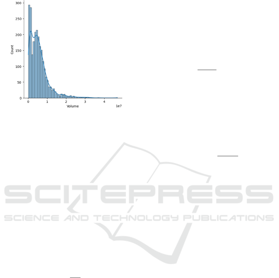
Figure 1: Volume distribution map of dataset 1

(Photo/Picture credit: Original).

A simpler preprocessing of the data allows to obtain

a more readable descriptive statistic, and no objective

factors must be encoded.

2.1.2 Data Cleaning

It is feasible to determine whether the dataset contains

null values by using the isnull function. The outcome

shown in this part indicates that there are no null

values, and the dataset is extremely well complete.

Nulls and duplicates can be removed to get a full

dataset suitable for machine learning.

2.1.3 Z-score Standardization

Z-score standardisation can adjust the dataset mean to

0, and standard deviation to 1. The standardisation

formula is as follows, where 𝜇 is the mean and 𝜎 is

the standard deviation.

𝑥









(1)

After normalisation, the data distribution needs to

be verified to ensure that the normalisation process

has not introduced bias or lost important information.

2.1.4 Interpolation

Due to its versatility and ease of calculation, simple

linear interpolation is a fundamental technique

utilized in many domains. It estimates unknown data

points by using a linear connection between known

data points, particularly when data gathering is erratic

or contains missing values. In real business cases,

data sets are often multivariate. Simple linear

interpolation can also be used for this situation.

Suppose the dataset is 𝑥



, 𝑦



 , which 𝑥





𝑥









, 𝑥









, 𝑥









,…,𝑥





 is multi-dimensional

eigenvector，𝑦



is the corresponding output value.

According to the datasets, located the interpolation

points as 𝑥𝑥







, 𝑥







, 𝑥







,…,𝑥



 , and find

nearest data point



𝑥



, 𝑦





and 𝑥



, 𝑦



.

For each dimension 𝑗𝑗  1,2,3, … , 𝑛 , use

interpolation formula:

𝑦𝑦

























𝑥







𝑥





 (2)

The final interpolated values are obtained by

combining the results of this formula, which is

applied individually on all dimensions. The weighted

average of the interpolated values for these

dimensions may be used to get the final y value

because the interpolated results for each dimension

are estimates. The weighted average weights may be

determined by other pertinent parameters or by the

precision of the dimensions' interpolation. a weighted

formula like this one:

𝑦





∑













∑









(3)

where 𝑤



is the weight of dimension j, 𝑦



is the output

value of dimension j.

2.2 Machine Learning Model Building

2.2.1 Feature Selection

In this stage, the data is first normalized after the

training and test sets have been divided.

Subsequently, the classifier for training is defined

using the LGBMClassifier, and the stepwise features

are selected using the SFS function. For many years,

feature selection has been a popular pre-processing

step. Numerous research works have highlighted the

value of feature selection in machine learning.

According to Virvou, Tsihrintzis, and Jain (Virvou et

al., 2022), feature selection improves classification

accuracy while reducing the size of the challenge.

Metrics called features are used to characterize

pertinent details about a data item. According to

Theng and Bhoyar, choosing the appropriate features

is a crucial stage in the construction of machine

learning models as it may greatly increase

performance and decrease model complexity (Theng

& Bhoyar, 2024). The initial purpose of stepwise

feature selection was to fit linear regression models.

With this method, any feature may independently

enter or exit the regression model (ibid.). This

approach has several drawbacks. To assess particular

characteristics, this technique first employs many

repeated hypotheses (ibid.). The selection of features

ECAI 2024 - International Conference on E-commerce and Artiﬁcial Intelligence

400

may result from this. Furthermore, Engelmann notes

that choosing the incorrect variables and experiencing

instability are potential risks associated with this

conventional feature selection approach (Engelmann,

2023).

The Stepwise Feature Selector (SFS) from

"mlxtend" is used for feature selection in this Python-

based study. The dataset was divided using

StandardScaler, and the classification model was

trained using LGBMClassifier. The variables

underwent a step-by-step process of feature selection,

and the significance of each variable to the model, as

well as the variation in accuracy at each stage, were

displayed.

2.2.2 Baseline Model and Comparison

Several methods have been initially shown to build

the baseline model before model optimization. This

project makes use of the following algorithms:

XGBoost, gradient boosting, logistic regression,

decision tree, K closest neighbors, random forest,

gaussian naive Bayes, light GBM, and neural

network.

Based on the comparison results of the base

models, this study selects the top 3 models and tuning

parameters. The subsequent analysis will be based on

these three algorithms for model optimisation.

2.2.3 Model Tuning

Once have identified the three best-performing

models, this study proceeds with model tuning. The

project defines two functions: get_paramslist and

param_search. Get_paramslist generates all possible

parameter combinations. Param_search loops

through all generated parameter combinations and

returns the best parameters based on the results of the

parameter tests.

2.2.4 Model Stacking and Model

Evaluation

In this project, the basic models are compared, and

then a stacking model is built to incorporate the

benefits of several models. The stacking model is an

integrated learning technique that combines the

predictions from several base models to enhance

overall prediction performance. Using the strengths

of many models to minimize the bias and variance of

a single model improves the overall accuracy and

resilience of the stacking model. The meta-learner of

the stacked model in this project is XGBClassifier,

with a maximum depth of 3. To assess the stacked

model's cross-validation performance, the

calculate_cv_scores function is utilized. To further

enhance the stacked model's performance, parameter

adjustment was done. This study created a parameter

grid with the following values: subsample percentage

(subsample), maximum depth (max_depth), and

learning rate (eta). This study then conducted a search

using these parameter combinations. Using a brute-

force search, the param_search function is used to

determine the ideal combination of parameters.

Continue to employ cross-validation during the

search, with the KS value serving as the assessment

criterion. Next, discovered the ideal combination of

parameters and deduced the matching ideal score.

Lastly, save the stacked model's ideal parameters and

scores in tuned_summary.

2.2.5 Hold-Out Set Test

In machine learning, a Hold-Out Set is a randomly

separated subset from the original dataset that is not

involved in the model's training process but is used to

test the model's performance on unseen data. The

primary purpose of this method is to assess the

generalization ability of the model, i.e. the model's

ability to handle new data (Berry et al., 2020). If the

performance of these models on the hold-out set is

consistent with the training set, which is suitable

proof that they are not overfitting, have good

generalization ability, and can provide reliable

predictions in real applications.

3 RESULTS

3.1 Stepwise Feature Selection

By choosing suitable characteristics, the model's

efficiency may be enhanced, the computational

burden can be decreased, and the occurrence of

overfitting can be avoided. Based on the stepwise

feature selection report (Figure 2), the model

performance shows varying patterns as the number of

features increases. When a single feature is chosen,

the model's performance is diminished, about at 0.78.

Nevertheless, when the amount of features is

augmented to two, the model's performance

experiences a substantial enhancement, reaching

around 0.79. This implies that the second feature has

a crucial impact on enhancing the model's

performance, presumably due to its provision of

significant supplementary information. From the

third feature onwards, the model's performance

reached a plateau, hovering consistently around 0.79

without any notable increase. The chart's blue-

coloured sections depict the potential variations in the

Irregular Stock Data Prediction Performance Optimisation Based on the Simple Linear Interpolation

401

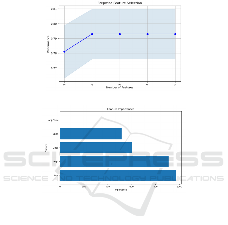
Figure 2: Stepwise feature selection

report

(Photo/Picture credit: Original).

Figure 3:

Feature

importance report (Photo/Picture credit: Original).

model's performance, typically called confidence

intervals. As the quantity of characteristics grows, the

shaded region expands, signifying heightened

ambiguity in performance. This behaviour might be

attributed to introducing more characteristics, which

may result in increased noise or excessive complexity

of the model.

The Figure 3 indicates that variables such as Low

and High exert a more pronounced impact on the

model. Previous analysis suggests that if the model's

performance is suboptimal, the data noise can be

reduced by deleting a few variables that have a

comparatively lesser influence. This enhances the

model's stability and performance.

3.2 Baseline Model Comparison

After building baseline models for many algorithmic

models, the following findings were found shown in

Table 2. The outcomes of machine learning (KS) are

assessed in this study under three criteria: accuracy,

area under the curve (AUC), and Kolmogorov-

Smirnov statistic. One of the easiest evaluation

measures to understand is accuracy, which is defined

as the proportion of samples the model appropriately

predicts generally (Silhavy & Silhavy, 2023). % of all

the samples for which the model generated accurate

forecasts. Although accuracy is generally used and

easily understood, in datasets with unequal

distribution of categories it often generates deceptive

findings. Accuracy is a less consistent metric than

AUC that tests the model's capacity to distinguish

positive from negative categories (Yang & Ying,

2022). On the AUC scale—which spans 0.5 to 1—a

higher score indicates a more discriminating model.

Since AUC is based on rankings rather than absolute

numbers, it is more representational than accuracy in

many cases and resists category imbalance (Yang &

Ying, 2022). Many times, the ability of a model to

ECAI 2024 - International Conference on E-commerce and Artiﬁcial Intelligence

402

discriminate between binary classification tasks is

evaluated using Kansas. The model distinguishes

between the two groups better the higher the KS

value. It gauges the largest difference between the

positive and negative categories' cumulative

distribution functions as anticipated by the model. An

essential nonparametric statistical test for assessing

machine learning models and contrasting

distributions is the Kansas test. Kolmogorov and

Smirnov initially suggested the KS test in 1933 and

1939 (Dodge, 2008). Kolmogorov and Smirnov

initially introduced it in 1933 and 1939 with an eye

toward comparing two sample distributions or

between a sample and a reference distribution. The

KS statistic is applied in machine learning to assess

the capacity of a classification model to distinguish

across numerous sample classes. The largest

variations in the cumulative distribution functions of

the positive and negative categories are discovered by

the KS test (Cong et al., 2021). Since the capacity of

the model to discriminate between positive and

negative samples rises with increasing maximal

difference, the higher the KS value, the better the

model's ability to do so.

This study chooses the three algorithms that have

the best KS performance in the baseline model. This

is so because the KS statistic directly measures the

model's capacity to discriminate between positive and

negative class samples (Dodge, 2008). On the other

hand, AUC is an overall sort-based statistic that could

not accurately reflect the model's ability to

discriminate over certain intervals, whereas accuracy,

while obvious, might yield misleadingly high results

on datasets with unbalanced categories. For the

Dataset in this research, Random Forest, XGBoost,

and K-Nearest Neighbors were chosen based on the

baseline model result.

3.3 Model Performance Evaluation

3.3.1 Model Result

The results are shown in the Table 3 below. The

model performs better when using the interpolation

technique. However, the effect varies according to the

particular model and measurements applied. Using

the SLI approach results in a little increase of 0.05%

and 0.92% in the accuracy and AUC measurements

under the XGBoost model.

Following SLI, the Random Forest model's

performance significantly improved in comparison to

XGBoost. While these measures increased by 1.06%

and 0.11%. This shows that the Random Forest model

may perform much better through interpolation, and

that it is more sensitive to the quality of the data.

Table 2: Dataset Baseline Model Result.

Model Accuracy AUC KS

Random Fores

0.835 0.907 0.688

XGBoos

0.824 0.909 0.668

K Nearest Neighbors 0.812 0.901 0.654

Light GBM 0.804 0.901 0.652

Gradient Boosting 0.807 0.900 0.645

Decision Tree 0.813 0.894 0.638

eural Networ

0.782 0.872 0.606

Logistic Regression 0.703 0.824 0.564

Gaussian Naive Bayes 0.717 0.803 0.564

Table 2: Model performance.

Data Type Base Data Simple Linea

Interpolation

Model Accuracy AUC KS Accuracy AUC KS

XGBoos

0.8344 0.9130 0.6906 0.8349 0.9214 0.6909

Random

Fores

0.8240 0.9081 0.6733 0.8357 0.9169 0.6873

K Nearest

hbors

0.8209 0.8209 0.8209 0.8357 0.8357 0.8357

Stacking

Model (XGB)

0.7691 0.8436 0.6229 0.8232 0.9071 0.6699

Irregular Stock Data Prediction Performance Optimisation Based on the Simple Linear Interpolation

403

Similarly, the K Nearest Neighbors model

displayed interpolation processing sensitivity. The

model improves all three measures by around 1.79%

under SLI. This increase in consistency shows that

when working with more full data, the KNN model is

more adept at capturing connections between

variables. The Stacking Model's performance yields

the most noteworthy outcome. The model's accuracy

increased by 7.03%, its AUC by 7.52%, and its KS

value by an even higher 7.55% when using the SLI

technique.

The intricate structure of the stacked model may

be the reason for its notable improvement. Greater

predictive ability is achieved by the stacked model,

which integrates the predictions of several underlying

models. But because of its intricacy, the model is also

extremely sensitive to the quality of the input. By

smoothing out missing values or irregular points in

the data, simple linear interpolation greatly increases

data consistency, which in turn greatly enhances the

stacking model's overall performance.

3.3.2 Findings and Discussion

The application of simple linear interpolation

improved the performance of all four models,

especially the stacked model (XGB), which showed

significant improvements in all metrics. This suggests

that stacked models, which combine multiple

algorithms, may be particularly sensitive to

improvements in data quality, while interpolation

methods can significantly improve data integrity and

consistency.

For integrated methods like XGBoost and

Random Forest, the performance gains remain

consistent, albeit more modest. This suggests that

while these models are already inherently robust in

dealing with missing data, their performance can still

be further improved by data preprocessing steps such

as interpolation. The improvements in the AUC and

KS metrics suggest that simple linear interpolation

can help to improve the discriminative power of the

model, leading to more accurate classification.

The K Nearest Neighbours (KNN) model showed

uniform improvements in all metrics, suggesting that

interpolation can enhance the performance of models

based on neighbourhood computation by providing

more complete data. However, the AUC

improvement was small, suggesting that despite the

help of interpolation, KNN is less sensitive to data

enhancement compared to more complex models

such as integrated methods or stacked models.

Overall, these findings emphasise the importance

of data preprocessing, particularly interpolation

methods, in improving the performance of machine

learning models. The consistent improvement across

all models suggests that applying simple linear

interpolation is an effective strategy to enhance

models' overall accuracy, AUC, and KS statistics

when dealing with datasets with missing or irregular

values. However, the magnitude of improvement also

suggests that model choice plays a vital role in the

benefits of interpolation. More complex models, such

as stacked models, may benefit more from

interpolation because they rely on the completeness

and consistency of the input data. On the other hand,

relatively simple models such as KNN or Random

Forest may see less gain.

3.4 Hold-Out Set Test

The hold-out set test results for this study are shown

in Table 4. Most of the results are relatively consistent

with the performance of the training set, and the AUC

and KS scores are stable with little variation. For the

XGBoost model, all metrics improved after applying

simple linear interpolation. This improvement

suggests that interpolation may have effectively

reduced noise in the data, allowing the model to better

capture the overall pattern of the data rather than the

noisy features, thus improving performance on the

retained set. This suggests that XGBoost benefits

from the interpolation process in preventing

Table 3: Dataset 1 Hold-Out Set Test Result.

Baseline SLI

Model Accuracy AUC KS Accuracy AUC KS

XGBoos

0.845 0.919 0.708 0.850 0.932 0.715

Random Fores

0.845 0.916 0.703 0.852 0.929 0.722

K Nearest Neighbors 0.831 0.912 0.690 0.835 0.914 0.684

Stacking Model (XGB) 0.773 0.774 0.549 0.858 0.924 0.716

ECAI 2024 - International Conference on E-commerce and Artiﬁcial Intelligence

404

overfitting and maintains a high predictive power on

unseen data. The Random Forest model shows a

similar trend with the application of interpolation,

especially when the KS values are improved

significantly. For the KNN model, despite the small

improvement in accuracy and AUC, the decrease in

KS values may suggest that the model faces

challenges in preventing overfitting. The KNN model

relies on local neighbourhood information, and

interpolation may have introduced some local biases

that do not represent the global pattern of the data,

which leads to a decrease in the model's ability to

generalise on new data. As the risk of overfitting is

closely related to model complexity, KNN being a

simpler model, the local noise introduced by

interpolation may cause the model to perform less

well than expected on the retained set.

The stacked model showed the most significant

performance improvements, especially in the AUC

and KS values. These significant improvements

suggest that simple linear interpolation greatly

reduces the random noise in the data, allowing the

stacked models to better learn and generalise the

global features of the data. For such complex models,

the improvement in interpolation processing helped

them to perform better on the retained set, suggesting

that interpolation not only helped to prevent

overfitting but also enhanced the generalisation

ability of the model.

4 LIMITATIONS AND FUTURE

PROSPECTS

While the study demonstrates that SLI can enhance

model performance, it is important to acknowledge

certain limitations. First and foremost, this study just

concentrates on data pertaining to a solitary stock

(Tesla), hence limiting its applicability to other stocks

or financial instruments. The data attributes of the

Tesla stock, such as volatility and trading volume,

might impact the reliability of SLI, and hence, the

outcomes may vary for equities with distinct trading

patterns or in diverse market circumstances.

Secondly, the study chose four models (XGBoost,

Random Forest, k-nearest Neighbors, and Stacking

Model) based on a comparison of baseline models.

The study did not investigate the effect of SLI on

other potentially pertinent models, such as neural

networks or other integration methods, which may

exhibit distinct responses to interpolation techniques,

despite the fact that these models encompass a range

of machine learning methodologies. Furthermore, the

study exclusively employed Accuracy, AUC, and KS

as performance indicators. Although these indicators

are often used and significant, they do not encompass

all facets of model performance. Metrics like as

Precision, Recall, and F1 Score can offer valuable

insights when working with highly imbalanced data,

a regular occurrence in financial markets.

Regrettably, the study does not thoroughly

investigate the overfitting problems that may arise

from SLI. Although SLI might enhance the

consistency of data, it can also generate artifacts that

some models may overfit, particularly in models such

as K-nearest neighbors that are sensitive to the local

structure of data. Additional examinations, such as

cross-validation and evaluation on data that was not

used during training, are required to verify that the

reported improvements in performance are not only a

result of overfitting.

5 CONCLUSION

This study investigates the impact of linear

interpolation on the effectiveness of machine learning

predictive models for stock data based on Tesla stock

data. Stepwise feature selection was used to optimise

the model. Also, Logistic Regression, Decision Tree,

K Nearest Neighbors, Random Forest, Gaussian

naive bayes, Light GBM, XGBoost, Gradient

Boosting, and Neural Network were used for

prediction, and the three algorithms with the best

results were selected for parameter tuning.

The results

show that SLI improves model accuracy, as well as

AUC and KS statistics to a certain extent, especially

on stacked models and integration methods that

exhibit significant performance gains. This suggests

that SLI, as a data preprocessing technique, can

enhance the predictive power of models by improving

data consistency and completeness. However, the

study also reveals that SLI's effect is inconsistent

across different models and data characteristics,

especially in contexts where overfitting may be

triggered, and SLI needs to be applied with more

caution. Also, this study has the limitation of having

a single set of data and a small number of model

choices. Nevertheless, the results of this study

provide necessary empirical support for the

application of SLI in financial data modelling,

highlighting the crucial role of data preprocessing in

enhancing the performance of machine learning

models.

Irregular Stock Data Prediction Performance Optimisation Based on the Simple Linear Interpolation

405

REFERENCES

Berry, M. W., Mohamed, A. H., & Wah, Y. B.

2020. Supervised and unsupervised learning for data

science. Springer.

Chopra, R., & Sharma, G. D. 2021. Application of artificial

intelligence in stock market forecasting: A critique,

review, and research agenda. Journal of Risk and

Financial Management, 14(11), 526.

Claerbout, J. F. 2004. Prediction-error filters and

interpolation. Stanford Exploration Project.

Cong, Z., Chu, L., Yang, Y., & Pei, J. 2021.

Comprehensible counterfactual explanation on

Kolmogorov-Smirnov test. Proceedings of the VLDB

Endowment, 14(9), 1583–1596.

Dodge, Y. 2008. Kolmogorov–Smirnov test. In The concise

encyclopedia of statistics (pp. 283–287). Springer.

Engelmann, B. 2023. Comprehensive stepwise selection for

logistic

regression. arXiv. https://arxiv.org/abs/2306.04876

Gao, J., An, Z., & Bai, X. 2022. A new representation

method for probability distributions of multimodal and

irregular data based on uniform mixture model. Annals

of Operations Research, 311(1), 81-97.

Gong, X., Chen, S., & Jin, C. 2023. Intelligent

reconstruction for spatially irregular seismic data by

combining compressed sensing with deep

learning. Frontiers in Earth Science, 11, Article

1299070.

Li, J., & Heap, A. D. 2014. Spatial interpolation methods

applied in the environmental sciences: A

review. Environmental Modelling & Software, 53, 173-

189.

Liapis, C. M., Karanikola, A., & Kotsiantis, S. 2023.

Investigating deep stock market forecasting with

sentiment analysis. Entropy, 25(2), 219.

Manousopoulos, P., Drakopoulos, V., & Polyzos, E. 2023.

Financial time series modelling using fractal

interpolation functions. AppliedMath, 3(3), 510-524.

Miles, R. E. 1981. Delaunay tessellation. The Computer

Journal, 24(2), 167-

172. https://academic.oup.com/comjnl/article/24/2/167

/338200

Nti, I. K., Adekoya, A. F., & Weyori, B. A. 2020. A

systematic review of fundamental and technical

analysis of stock market predictions. Artificial

Intelligence Review, 53(4), 3007-3057.

Sambridge, M., Braun, J., & McQueen, H. 1995.

Geophysical parametrization and interpolation of

irregular data using natural neighbours. Geophysical

Journal International, 122(3), 837-857.

Shukla, S. N., & Marlin, B. M. 2021. Multi-time attention

networks for irregularly sampled time

series. arXiv. https://arxiv.org/abs/2102.02197

Silhavy, R., & Silhavy, P. 2023. A review of evaluation

metrics in machine learning algorithms. In Artificial

intelligence application in networks and systems (Vol.

724, pp. 15–25). Springer.

Theng, D., & Bhoyar, K. K. 2024. Feature selection

techniques for machine learning: A survey of more than

two decades of research. Knowledge and Information

Systems.

Virvou, M., Tsihrintzis, G. A., & Jain, L. C. (Eds.).

2022. Learning and analytics in intelligent systems:

Advances in selected artificial intelligence areas (Vol.

24).

Weerakody, P. B., Wong, K. W., Wang, G., & Ela, W.

2021. A review of irregular time series data handling

with gated recurrent neural networks. Neurocomputing,

441, 161-178.

Xin, S., Wang, P., Xu, R., Yan, D., Chen, S., Wang, W.,

Zhang, C., & Tu, C. 2023. SurfaceVoronoi: Efficiently

computing Voronoi diagrams over mesh surfaces with

arbitrary distance solvers. Communications of the

ACM.

Yang, T., & Ying, Y. 2022. AUC maximization in the era

of big data and AI: A survey. ACM Computing Surveys,

55(8).

ECAI 2024 - International Conference on E-commerce and Artiﬁcial Intelligence

406