Implementation of the State-of-The-Art Results for Sales Prediction

Tianyi Chen

School of Mathematics and Physics, North China Electric Power University, Beijing, China

Keywords: Sales Prediction, Machine Learning, LSTM, ARIMA.

Abstract: Sales prediction is a projection into the future of expected demand, given a stated set of environmental

conditions. It is an integral part of a critical process for matching demand and supply in many companies.

Within this text, the topic focuses on the latest domestic and overseas research advances in this domain with

prospects and visions for future development. Besides the traditional tools in time series analysis, e.g., the

Auto-regressive Integrated Moving Average Model (ARIMA), more Machine Learning (ML) based methods,

such as the Long Short-term Memory Network (LSTM) and other Neural Networks (NN), are demonstrating

their strong prediction power and are increasingly being applied into hybrid models, which integrate them

with the former statistical models. However, with more applications of such ML-based techniques, their lack

of explainability is uncovered, causing their low acceptance by decision-makers. Thus, more work is needed

to examine the optimization of sales planning with more innovative and customized strategies under the

guidance of accurate forecasts. These results serve as an elementary reference to inspire future exploration in

this hot spot.

1 INTRODUCTION

Predictions of future sales are crucial for corporate

planning, and the major uses of sales forecasts

frequently include setting production schedules,

budgeting capital, and allocating resources to

marketing strategies (Douglas, 1975). Since the

significance of accurate sales forecasting to business

success has become widely recognized, considerable

efforts have been expended on the continuous

development of Sales prediction for more than

seventy years. Dating back to the 1950s, a possibly

novel approach of sales forecasting utilizing sampling

embraced its rapid maturity from its infancy

attributed to the success of the predictions based on

the Federal Reserve Board’s Survey of Consumer

Finances. Nevertheless, forecasting sales using

sample surveys has drawbacks that should be

considered in determining whether the approach is

feasible in certain cases compared to other methods.

Among these factors, expense is a vital aspect.

Sampling is often performed by personal interviews.

Hence, it is undoubtedly one of the most expensive

ways for sales prediction. Although its exponents

held the view that the costs of sampling could be

https://orcid.org/0009-0003-2958-9760

ignored compared with the value created for future

revenues, the fact indicated that most small consumer

goods companies were unlikely to prioritize sampling

and incur those expenses when more alternatives

were cost-effective. On the other hand, in the cases of

predicting sales of industrial products such as heavy

machinery, manufacturers usually sell their products

directly to their end-users (Robert, 1955). Under this

circumstance, time-consuming interviews can be

completed with calls from salespeople in a smoother

process, thereby making sampling a conditionally

useful method of sales forecasting.

Subsequently, the expense factor was no longer a

fundamental issue because obtaining the required

data to conduct studies was much more effortless due

to the greater availability of those powerful tools -

computers and necessary software. Since the last ten

years have seen phenomenal progress in processing

Big Data, sampling gradually lost its advantages with

the advent of emerging techniques. Fortunately, it

maintains its position in subjective forecasting on

potential demands in durable commodities and new

products. In addition, similar methodologies are still

playing their roles in Social Sciences. In survey

research, information from a sample of individuals is

324

Chen, T.

Implementation of the State-of-The-Art Results for Sales Prediction.

DOI: 10.5220/0013225000004568

In Proceedings of the 1st International Conference on E-commerce and Artiﬁcial Intelligence (ECAI 2024), pages 324-330

ISBN: 978-989-758-726-9

normally gathered through interviews and systematic

sampling. Organizational and administrative

capacities are also necessary for survey research, and

these can be typically provided by nonprofit survey

centers or commercial survey companies (Byrne et al.,

2011). During the past decades, sales prediction has

been extensively studied, and more than two hundred

different forecasting methods have been developed.

Unstable business conditions have had negative

impacts on their performance, while such adverse

effects have improved by incorporating sophisticated

computer technology as well as mature statistics

theories. In general, forecasting techniques can be

categorized into two types, i.e., qualitative and

quantitative approaches. Representative qualitative

prediction means involve Brainstorming (BS), the

Delphi technique (Linstone, 1985), and subjective

probability estimates (Wallsten et al., 1997). They all

recognize the contribution of experienced managers,

experts, salespeople, and consumers through several

rounds of discussions concerning analysis, reasoning,

and judgment because it would have been virtually

impossible to gather and research all the information

(Byrne et al., 2011).

In contrast, quantitative methods are more

reusable but less flexible. Models can be built with

raw historical data based on mathematical statistics

theories. The regression analysis has undoubtedly

retained its dominance in finding correlations such as

causal relationships between factors especially when

changes in the unit period are irregular within an

explicit overall trend. Because of the time sequence

nature of sales series, the time series analysis

achieved a dramatic growth in popularity. Both

methodologies are capable of tackling multivariate

complex problems with numerous factors inside via

corresponding multiple models. Given the different

properties of historical data, various models have

their applicable scenes. For instance, despite its

restrictions in capturing non-linear relationships and

processing non-steady time-series data, the Auto-

Regressive Moving Average Model (ARMA)

performs well in stationary time-series forecasts.

Some models apply to data with seasonal trends and

other regular changes in short-term or long-term

periods (Huang et al., 2015). It should be noted that

the subjective and objective ways are not isolated but

complementary. The practice has proved that

combining outperforms using separately. Currently,

advanced programming languages such as Python

and R can realize those analyzing work efficiently.

Recently, when accuracy has been increasingly

regarded as the central problem of sales prediction,

more established methods have chosen to employ

Machine Learning (ML) algorithms as the key

technique for more effective forecasts. Independent

variables including time-series sales data and factors

potentially influencing future sales are inputted into

models based on those ML algorithms to output the

target variables such as future sales (Huang et al.,

2015). Those models, for example, Artificial Neural

Networks (ANNs), are better able to handle nonlinear

problems with good precision and lower error.

Instead of merely optimizing a single model, more

complicated models combine at least two individual

algorithms to raise accuracy. However, over-fitting is

a current challenge for optimization.

Contemporarily, in this evolving field of human

endeavor, it is the objective of this paper to expose

previous research that has been undertaken,

summarize what has already been discovered, reflect

the existing issues, and explore its future paths. The

rest of this document is organized as follows. Section

2 provides a detailed interpretation of sales prediction.

Then, Section 3 introduces two classic models - the

ARIMA model and the LSTM network. To explore

their implications, Section 4 focuses on the most

cutting-edge research applying these models. In

Section 5, insights into limitations and development

direction are presented, and future projects are

proposed. Ultimately, Section 6 takes charge of the

conclusion, summarizing the covered topics.

2 DESCRIPTIONS OF SALES

PREDICTION

Sales prediction refers to a process in which

enterprises, based on full investigations of existing

information, the characteristics of different products,

and historical data, apply scientific methods to carry

out multi-angle and all-round analyses for various

factors that affect sales and disclosing the inherent

discipline of the needs of the market, thus making

relatively accurate estimations of the sales volume

and its development trends that the companies may

achieve in a specified period of the future. Briefly,

sales prediction is to forecast the unknown consumer

demand for numerous products in the future market

according to past and present known information

(Yang et al., 1985).

The generalized sales prediction also includes a

market survey, which represents the critical basis for

predicting sales volume. A market survey is defined

as the process of concluding whether there is a real,

potential, or future market for the product as well as

the size of the market by understanding the supply

Implementation of the State-of-The-Art Results for Sales Prediction

325

and marketing conditions in various types of markets

related to a specific product (Cao & Zhu, 2004). Sales

prediction is an important part of business planning

management and sales management. Its function is

mainly reflected in the following two aspects. First, it

guides and improves the marketing strategies of

targeted products based on forecasts to strive for

lifting sales. Second, it helps determine informed

production plans to avoid out-of-stock and excessive

supply, and ultimately promote sales. Sales prediction

can be divided into two categories. One is short-term

sales prediction, which refers to forecasts within a

year, quarter, or month. The other is long-term sales

forecasting, which refers to projections for over one

year. Short-term prediction can be further classified

into normal sales forecasting and seasonal sales

forecasting where sales are subject to seasonal

variation.

In addition to simply projecting demand

quantities in the future, further efforts can be put into

forecasting profit, cost, and funds. Profit Forecasting

refers to the process of expecting and conjecturing the

possible profit levels and their trends of change, based

on the prediction of sales volume, the enterprises’

aims for future development, and other relevant

factors. Concretely, it includes forecasts on target

profit, profit sensitivity, and profit analysis under risk

conditions, etc. (Cao & Zhu, 2004).

Cost prediction is the process of using special

methods to evaluate future cost levels and their

evolving trends according to the companies’ future

development goals and objective profits. It is

primarily composed of forecasts on target cost, cost

of the best product quality, and the trends of

development of the cost levels of the products, etc.

Fund Forecasting, also named funding requirement

forecasting, is defined as speculating the amount, the

source channels, directions of the application, and

effects of funds that enterprises need over a certain

period in the future by specific techniques, based on

sales prediction, profit forecasting, cost prediction,

the future developing objects, and various factors

affecting fund. It mainly contains the requirement of

liquidity, the fund supplements, and the fixed assets

investment projects.

Sales prediction is a convoluted issue. Apart from

pondering on many factors, the salient complexity in

their relationships needs to be carefully analyzed.

Therefore, their impacts on sales must be considered

synthetically. Furthermore, when forecasting, based

on the features of given products, factors should be

distinguished between primary and secondary, while

proper forecasting methods should be selected. These

factors can generally be classified into internal factors

and external factors. External factors influencing

sales consist of (Chen, 1987):

 The current market environment;

 The market share of enterprises;

 The economic development trends;

 The competitors’ situation.

Internal factors that affect sales include:

 Past sales volume;

 The prices of the products;

 Product functionality and quality;

 Supporting services provided by companies;

 Advertising and other various sales-

promotion methods;

 The production capacity of the enterprises.

3 MODELS FOR SALES

PREDICTION

3.1 ARIMA

Under the assumptions of linear relationships, all of

the fascinating dynamics within a time series usually

cannot be adequately explained by conventional

regression. Instead, the auto-regressive (AR) and

ARMA models have been proposed as a result of the

introduction of correlation generated through lagged

linear relations (Shumway & Stoffer, 2017). In terms

of the non-stationary scenarios, ARIMA models have

substantially improved the fitting precision of non-

stationary sequences. Since Box and Jenkins put

forward this model in 1970, it has become the most

classic model for fitting time series (Wang, 2020).

The difference operation has the powerful capability

of extracting assured information. Many non-

stationary time series display the properties of

stationary sequences after difference, and these non-

stationary ones are called differential stationary series,

which can be fitted by ARIMA models.

An auto-regressive integrated moving average

model, abbreviated ARIMA(p, d, q), is of the

following form, where the ordinary auto-regressive

and moving average components are represented by

polynomials φ(B) and θ(B) of orders p and q.





𝐵



∇



𝑥



= Θ



𝐵



𝜖



𝐸



𝜖





=0,𝑉𝑎𝑟



𝜖





= 𝜎





, 𝐸



𝜖



𝜖





=0,𝑠≠𝑡

𝐸𝑥



𝜖



=0,∀𝑠< 𝑡

(1)

It is suggested that the essence of the ARIMA models

is the combination of different operations and the

ARMA models. Such a relationship is of great

significance for it means that if any non-stationary

series could achieve stationary through difference of

ECAI 2024 - International Conference on E-commerce and Artiﬁcial Intelligence

326

an appropriate d order, the ARMA models would be

used to fit this post-difference sequence. Since the

analytic methods for ARMA models are already well-

developed, analysis on differential stationary series

would also be highly feasible and reliable to carry out

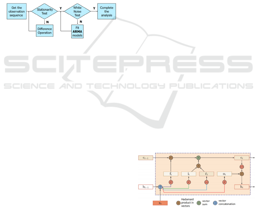
(Wang, 2020). Hence, after mastering the modeling

approach to the ARMA model, it is relatively easier

to try to model a given observation sequence via an

ARIMA model. It follows the following process

shown in Fig. 1. Based on the principles of the

minimum mean squared error (MMSE) forecasting,

the methods are similar when predicting an ARIMA

model and an ARMA model. After modeling the

original sequence, the fitted model can be directly

applied to the forecast. From modeling to prediction,

all the work can be realized using programming

languages.

Figure 1: The modeling procedure for ARIMA models

(Wang, 2020).

3.2 LSTM

Due to its neurons with self-feedback, a Recurrent

Neural Network (RNN) excels in processing time

series data of arbitrary length, such as video, speech,

and text. It appears special construction, prominent

short-term memory, facile learning approach, and

stunning non-linearity that former Neural Networks

(NN) have never done. In a common RNN, neurons

receive information not only from others but also

from themselves, forming network structures with

loops. Theoretically, RNNs are able to approximate

any nonlinear dynamical systems.

The parameters in an RNN can be learned by the

Back-Propagation Through Time (BPTT) algorithm,

namely a parametric learning algorithm passing the

error information forward step by step in reverse

chronological order. However, relatively long input

sequences can lead to the long-term dependency

problem, the Gradient Exploding Problem as well as

the Vanishing Gradient Problem. Among all the

advanced means to remedy these problems, importing

the Gating Mechanism ranks as the most effective

solution. The Gating Mechanism is designed to

control the accumulation speed of information by

selectively adding information while forgetting the

previously accumulated one (Qiu, 2020). This

improved type of RNN is called Gated RNN, which

includes the popular LSTM network. The memory

cell c is core to an LSTM network, where three gates

are responsible for specific tasks. The Forget gate f

determines how much information the previous

internal state c

t-1

needs to forget. The Input gate i

controls how much information the current candidate

state 𝒄



should save. While the Output gate o

could

decide how much information the current internal

state c

needs to output into the external state h

, the

hidden state in an RNN. The calculated approach of

the candidate state 𝒄



, the internal state c

, the external

state h

, and the three gates are as follows, where σ(x)

is the Logistic Function, W

, U

, and b

are all

learnable parameters as illustrated in Fig. 2 and

following (Qiu, 2020):

= σ(W

+ U

t-1

+ b

) (2)

= σ(W

+ U

t-1

+ b

) (3)

= σ(W

+ U

t-1

+ b

) (4)

𝐜



= tanh(W

+ U

t-1

+ b

) (5)

= f

⨀ c

t-1

+ i

⨀ 𝐜



(6)

= o

⨀ tanh(c

) (7)

From the structure of the recurrent unit of an LSTM

network depicted in the following figure and the

formulas listed above, the computational process can

be divided into three steps. First, work out the

candidate state 𝒄



and the three gates using the

previous external state h

t-1

and the current input x

Second, update the memory unit c

with the Forget

gate f

and the Input gate i

. Third, transmit the

information about the internal state c

to the external

state h

with the Output gate o

. The impact of the

LSTM networks has been notable in language

modeling, Speech Recognition, Natural Language

Generation (NLG), and other applications

(Sherstinsky, 2020).

Figure 2: The structure of the recurrent unit in the LSTM

networks (Qiu, 2020).

Implementation of the State-of-The-Art Results for Sales Prediction

327

4 IMPLEMENTATIONS AND

APPLICATIONS

In broad practical applications, many cases in recent

years have applied ARIMA models, LSTM networks,

and their variants integrating both models. When

implementing forecasts, their predictive objects are

often presented as time series. Time series, sequences

of historical observations at consistent intervals of

one or more variable(s), are usually analyzed for

purposes such as predicting the future based on past

knowledge, comprehending variables underlying the

generation of measured values, or just giving a

summary describing the conspicuous features of the

series (Swami er al., 2020).

In one project serving as a competition on the

Kaggle platform, competitors were asked to predict

the next month’s total sales of every product based on

their past daily sales data ranging from January 2013

to October 2015 for 1C Company, one of the largest

independent Russian software developers and

publishers.

In the provided table, columns such as item name,

item category, and shop ID, do not vary with time.

Variables like item count and item price, in contrast,

are time-dependent. In the paper of a group of

contestants, their work started with a series of studies

and discussions. Inspired by others, they finally

decided to try ARIMA and LSTM as learning

algorithms for this regression task.

Their next step was the traditional data pre-

processing - from tidying data, and exploratory data

analysis (EDA) that roughly grasped the general

distributive tendencies of the data, to the feature

engineering where they aggregated the total revenue

and total item_count_day for the month, computed

weighted mean price and average price, extract lags

of numeric features, and one hot encode ‘month’,

‘year’, ‘item_category_id’, ‘shop_id’. They split the

data set for the past 34 months into three subsets - 32

months for training, one month for validation, and

one month for testing. When deploying the ARIMA

method that works best for the univariate time series,

they group their training set according to identifier

columns and respectively fit their own ARIMA

models (Swami et al., 2020).

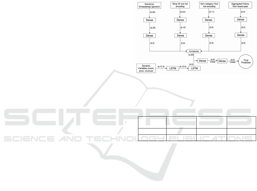
In Fig. 3, since the input contains both static and

dynamic features, they utilized an LSTM-based

neural network for the prediction, where the stacked

dense layers refer to the multiple layers of Fully

Connected Neural Networks (FCNN). Given the time

and resource limit, only batch size b and the L2

regularization coefficient λ shared by all layers were

taken into account when finding the optimal hyper-

parameters by Adaptive Moment Estimation (Adam)

optimizer and Mean-Squared Loss function (Swami

et al., 2020). Their final outcomes are listed in Table

1, where the criterion for evaluating the models’

performance is the Root Mean Square Error (RMSE).

Evidently, their LSTM-based network, where the

optimal b and λ are respectively 512 samples and

0.001, performed better than their ARIMA model

(Swami et al., 2020).

Figure 3: The LSTM based neural network architecture,

with batch size b and tanh activation function (Swami et al.,

2020).

Table 1: Comparing the performance of different models

(Swami et al., 2020).

Model Training

RMSE

Validation

RMSE

Test

RMSE

LSTM 0.804657 0.889786 0.92417

ARIMA 0.963426 0.982234 1.09266

Aside from the above one, similar comparisons

between these two statistical and Deep Learning (DL)

approaches have been executed in other papers. In a

profit prediction task, researchers struggled to

forecast the gross profit obtained for the next five

years. The sales data set comprises of 14 variables,

such as the item type, order date, the unit price and

the cost of each item type, and the total revenue, cost,

and profit with around 1 million records from 1972 to

2017. Align with Fig. 1, a requisite step is to check

the stationarity of the time series, commonly using the

Augmented Dickey-Fuller (ADF) test, and make

transformations when necessary, which is unique to

developing ARIMA models, compared with building

LSTM networks. Correspondingly, LSTM also

requires data normalization, handling different

attributes into dimensionless scalars. In this instance,

researchers choose to employ Min-Max Scaling

(Sirisha et al., 2022).

According to their results, their LSTM network

surpassed their ARIMA model with a good accuracy

of 97.01% and 93.84% (Sirisha et al., 2022). It has

ECAI 2024 - International Conference on E-commerce and Artiﬁcial Intelligence

328

been found that the accuracy of the LSTM model

randomly varied with epochs. Hence, the paper

advises readers to end the training process at the

minimum number of epochs once a respectable

precision is reached. When it comes to hybrid models,

in one recent paper, a group of researchers proposed

their novel solution to forecasting e-commerce sales

for a real-life store and then compared it against the

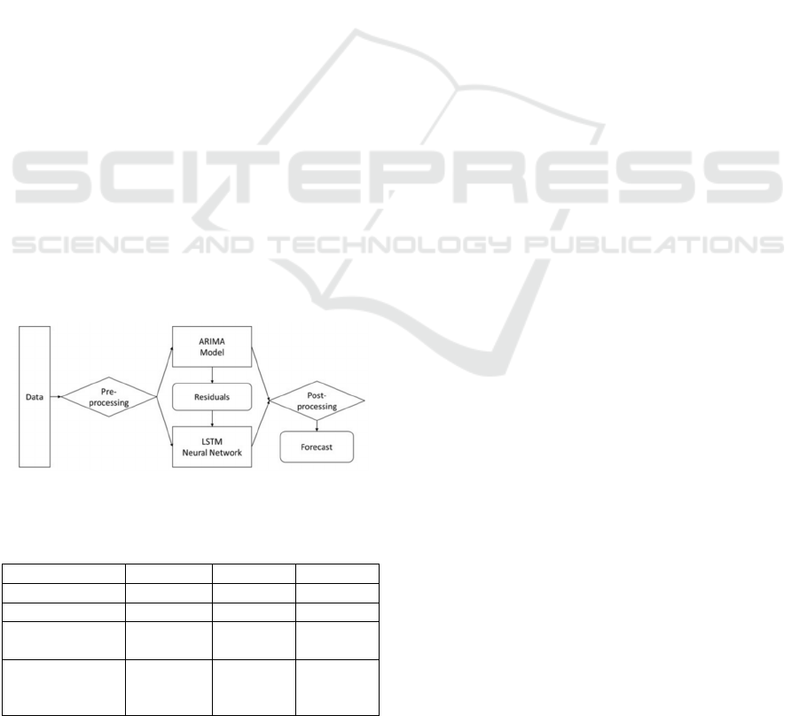
other three tested models. As illustrated in Fig. 4,

their hybrid model incorporates an ARIMA model,

which is responsible for predicting one-dimensional

time series data, and an LSTM network for fitting the

non-linear residuals of the former ARIMA model

together with the final retail price after discounts,

which can capture promotions and sales periods

(Vavliakis et al., 2021).

In their data set, there were sales data for 23,432

products in 1,418,480 order lines covering six years.

Two factors, the monthly average retail price and the

monthly amounts sold, were used for each product.

Before building the LSTM neural network, they

precisely tested the residuals, the difference between

the predicted and real values, to see whether they are

unrelated to each other and whether their mean value

is approaching zero. After conducting their

experiment for 50 random products, they respectively

calculated the three evaluation metrics for each

product, which are the Mean Square Error (MSE), the

RMSE, and the Mean Absolute Error (MAE). The

results are collectively shown in Table 2. Notably,

their ARIMA model and their LSTM network were

exceeded by their competing ones. Moreover, the

performance of their proposed model improved when

they considered the retail price.

Figure 4: Architectural diagram of the proposed solution

(Vavliakis et al., 2021).

Table 2: Comparing the evaluation results for 50 products.

Solution MSE RMSE MAE

LSTM 540.76758 13.2629 9.68830

ARIMA 466.05542 12.2340 9.21864

Proposed

Methodolog

415.44138 11.6794 8.88266

Proposed

Methodology

with Retail Price

412.74034 11.5222 8.73078

In another work on forecasting Indonesia’s local

exports one year ahead for governments, researchers

also trained a hybrid model, where the LSTM and the

ARIMA models separately assume predicting the

non-linear and linear components of the data (Dave et

al., 2021). Not surprisingly, this model managed to

outperform other standalone ones with the lowest

Mean Absolute Percentage Error (MAPE) of 7.38%.

As suggested above, a hybrid model typically

outstrips its separate ones in accuracy. To examine

the reason, it is important to note that mathematics

statistics models taking ARIMA models as represent,

are based on history records to analyze their long-

term trend, seasonal, cycling, and irregular effects

comprehensively. Whereas the ML-based methods

represented by the LSTM and other neural networks

mostly integrate other influencing factors, such as

selling prices, discounts, holidays, and weather, to

enrich its input and thus forecast as accurately as

possible (Fries & Ludwig, 2024).

5 LIMITATIONS AND

PROSPECTS

Looking back on the evolution of sales prediction,

great strides have been made in its theoretical

framework and a myriad of successful practices.

Meanwhile, the introduction of ML-based methods

has greatly enriched people’s choices of available

alternatives that can realize more accurate forecasts.

Accuracy indeed matters a lot in sales prediction.

Nevertheless, it ought to be borne in mind that the

ultimate purpose is to design wise marketing ploys

and lay out sound production plans while forecasting

just means. Without establishing a valid connection

between the chilling data and more active thoughts,

enterprises would fail to drive growth in revenue

during the next period. Accordingly, how to gain

strongly explainable outcomes and sink in their

implications through an ML-based forecast poses a

tremendous challenge.

Taking the baking industry, for example, Baked

goods, as the representative of Western cuisine, are

characterized by short shelf life, large material

wastage, a highly volatile demand, a qualified store

environment, and higher requests for food quality and

safety. To better reflect and address the newly arisen

problem in sales prediction, researchers have

investigated the use of ML-based techniques in a

medium-sized German bakery in a rural area. In their

findings, they found it difficult to explain their

accurate forecasting values properly. Although they

tried to visualize the correlations of various factors by

Implementation of the State-of-The-Art Results for Sales Prediction

329

drawing different graphs to interpret their results

preliminary, the owner and people working there

hardly accepted their conclusions and insisted their

focus on the website and the digital ordering process.

They even showed scepticism when prediction values

failed to meet their perceived expectations though

researchers stressed that their ideas were only

references (Fries & Ludwig, 2024).

Consequently, transparency and interpretability are

essential for unfolding the full potential of various

ML-based models because they ensure clear answers

to two basic questions regarding how the model

works and what the model implies (Fries and Ludwig,

2024). To resolve the trust issue, formulating more

targeted and convincing sales prediction schemes

based on these attractive approaches for diverse

industries would help.

6 CONCLUSIONS

To sum up, sales prediction is helpful in sales

planning to achieve sales at or near the level of

customer demand. It pertains to the proper use of

various techniques, both qualitative and quantitative,

within the context of corporate information systems.

The most efficient forecasting methods these days are

stochastic models and ML algorithms, such as

ARIMA, and LSTM, and their hybrid models that can

easily fetch linear and non-linear sales trends. In most

cases, a hybrid model tends to outperform its single

models by obtaining lower MSE or RMSE. For

example, an integrated LSTM-ARIMA model shows

higher accuracy than a single ARIMA model and an

LSTM-based network. Nevertheless, those intricate

ML-based models are often hard to explain in actual

applications, thus rarely fulfilling their role in making

practical plans. Therefore, despite the continual

innovation in more sophisticated methods, more

attempts to fill this gap are being urged to attain more

functional and informative forecasts. The present

article aims to motivate more follow-up practitioners

to enable sales prediction to keep evolving with the

times and satisfy the needs of more businesses.

REFERENCES

Byrne, T. M. M., Moon, M. A., Mentzer, J. T., 2011.

Motivating the industrial sales force in the sales

forecasting process. Industrial Marketing Management,

40(1), 128-138.

Cao, H., Zhu, C., 2004. Management Accounting. Tsinghua

University publishing house co., ltd.

Chen, Z., 1987. Management Accounting - Chapter IV

Sales Prediction. Shanghai Accounting, 9.

Dave, E., Leonardo, A., Jeanice, M., Hanafiah, N., 2021.

Forecasting Indonesia exports using a hybrid model

ARIMA-LSTM. Procedia Computer Science, 179, 480-

487.

Dalrymple, D. J., 1975. Sales forecasting methods and

accuracy. Business Horizons, 18(6), 69-73.

Ferber, R., 1955. Sales Forecasting by Sample Surveys.

Journal of Marketing, 20(1), 1-13.

Fries, M., Ludwig, T., 2024. Why are the sales forecasts so

low socio-technical challenges of using machine

learning for forecasting sales in a bakery. Computer

Supported Cooperative Work (CSCW), 33(2), 253-293.

Huang, W., Zhang, Q., Xu, W., Fu, H., Wang, M., Liang, X.,

2015. A novel trigger model for sales prediction with

data mining techniques. Data Science Journal, 14, 15-15.

Lawrence, M., Goodwin, P., O'Connor, M., Önkal, D., 2006.

Judgmental forecasting: A review of progress over the

last 25 years. International Journal of forecasting, 22(3),

493-518.

Linstone, H. A., 1985. The delphi technique. In

Environmental impact assessment, technology

assessment, and risk analysis: contributions from the

psychological and decision sciences. Berlin, Heidelberg:

Springer Berlin Heidelberg.

Qiu X., 2020. Neural Networks and Deep Learning. China

Machine Press.

Sherstinsky, A., 2020. Fundamentals of Recurrent Neural

Network (RNN) and Long Short-Term Memory (LSTM)

network. Physica D: Nonlinear Phenomena, 404,

132306.

Shumway, R. H., Stoffer, D. S., Shumway, R. H., Stoffer,

D. S., 2017. ARIMA models. Time series analysis and

its applications: with R examples, Springer, 75-163.

Sirisha, U. M., Belavagi, M. C., Attigeri, G., 2022. Profit

prediction using ARIMA, SARIMA and LSTM models in

time series forecasting: A comparison. IEEE Access, 10,

124715-124727.

Swami, D., Shah, A. D., Ray, S. K., 2020. Predicting future

sales of retail products using machine learning. arXiv

preprint arXiv:2008.07779.

Vavliakis, K. N., Siailis, A., Symeonidis, A. L., 2021.

Optimizing Sales Forecasting in e-Commerce with

ARIMA and LSTM Models. In WEBIST (pp. 299-306).

Wallsten, T. S., Budescu, D. V., Erev, I., Diederich, A.,

1997. Evaluating and combining subjective probability

estimates. Journal of Behavioral Decision Making,

10(3), 243-268.

Wang Y., 2020. Time Series Analysis with R. China Renmin

University Press.

Yang M., Rong Y., Wang S., 1985. Chapter V Sales

Forecasting Methods. Modern Finance And Economics

- Journal of Tianjin University of Finance And

Economics, 4.

Yu, Y., Si, X., Hu, C., Zhang, J., 2019. A review of

recurrent neural networks: LSTM cells and network

architectures. Neural computation, 31(7), 1235-1270.

ECAI 2024 - International Conference on E-commerce and Artiﬁcial Intelligence

330