Restaurant Revenue Prediction Using Machine Learning: A

Comparative Study of Multiple Linear Regression and

Random Forest Models

Yunmiao Wu

Department of Mathematics, Jinan University, Guangzhou, Chi

Keywords: Restaurant Revenue, Machine Learning, Multiple Linear Regression, Random Forest.

Abstract: As the food delivery industry develops, the restaurant sector is becoming increasingly competitive. To help

restaurant owners have a brief estimation on whether their restaurant can be profitable or not, it is crucial to

accurately predict restaurant revenue. In this paper, Multiple linear regression and random forest methods will

be used to predict restaurant sales. First, some brief data preprocessing will be made, and then the correlation

p-value will be calculated to select the numerical variables that are correlated with restaurant sales. Then,

multiple linear regression model will be used to evaluate the linear relationships between these features and

the target variable. The random forest model will also be applied. The result shows that the random forest

method outperforms the multiple linear regression method in terms of prediction accuracy when the feature

has a non-linear relationship with the restaurant revenue. This research could help the restaurant owners to

make their business strategies.

1 INTRODUCTION

In today's highly competitive restaurant industry, it’s

very important for the restaurant to maintain their

profitability. To achieve it, accurately predicting the

restaurant revenue becomes essential. Revenue

forecasting plays a critical role in a restaurant's future

planning for it can influence decisions on inventory

management, staffing, marketing strategies and

financial investments. However, predicting restaurant

sales is particularly challenging, since there are wide

range of factors that can influence it. Variables such

as location, customer demographics, average meal

price, marketing budget and even local economic

conditions can all impact sales, making traditional

forecasting methods less effective.

As the complexity of influencing factors

increases, more appropriate methods are needed to

better predict the revenue. This is where machine

learning can be used for its ability to process and

analyse large volumes of data, offering a powerful

solution for predicting restaurant sales. Unlike

traditional methods which may rely on simple linear

relationships or past trends, machine learning models

https://orcid.org/0009-0007-4040-1350

can capture complex, non-linear relationships

between multiple variables, providing more accurate

and reliable predictions.

A wide range of data points, such as the number

of reviews, weekly reservations, restaurant ratings,

and economic indicators can be incorporated into

predictive models by leveraging machine learning.

These models can learn from the data, identifying

patterns and relationships that may not be

immediately apparent. For instance, machine learning

can help us understand how factors such as a

restaurant’s rating or number of social media

followers influence the restaurant’s revenue.

Moreover, as more data becomes available, machine

learning models can improve its fitting performance,

leading to increasingly accurate predictions over

time. By applying these methods to predict restaurant

revenue, businesses can anticipate fluctuations in

revenue and adjust their strategies accordingly. This

proactive approach enables restaurant owners to

better estimate their profitability, reduce waste, and

cater more effectively to customer demands.

Wu, Y.

Restaurant Revenue Prediction Using Machine Learning: A Comparative Study of Multiple Linear Regression and Random Forest Models.

DOI: 10.5220/0013215500004568

In Proceedings of the 1st International Conference on E-commerce and Artiﬁcial Intelligence (ECAI 2024), pages 299-306

ISBN: 978-989-758-726-9

299

2 LITERATURE REVIEW

Predict restaurant revenue effectively has received

considerable attention in recent years. There exist

numerous studies using various machine learning and

statistical techniques to tackle this complex problem.

In these studies, they have highlighted the growing

interest in leveraging advanced computational

techniques to provide more accurate and reliable

financial forecasts, which are crucial for the

operational success of businesses in the restaurant

industry.

Siddamsetty et al. (2021) have predicted

restaurant revenue by using different machine

learning methods. their study evaluated the

effectiveness of several commonly used machine

learning algorithms in revenue prediction, including

Catboost algorithm and Random Forest algorithm,

and the typical regression models. The results

indicated that the Random Forest method and the

Catboost method could significantly improve

prediction accuracy compared with the traditional

Bayesian linear regression, especially when dealing

with large-scale, multidimensional datasets. This

study provides important insights into how to select

and optimize machine learning algorithms for more

efficient predictions.

Bera (2021) attempts to explore the topic from an

operational analytics perspective, studying the

application of machine learning algorithms in

predicting restaurant sales revenue. This study

focused on the importance of picking the truly

relevant feature, it also demonstrated how various

machine learning algorithms (such as random forests

and gradient boosting machines) can be used to

analyze and predict restaurant sales revenue. In the

study several ways are tried to compare and choose

the feature, like their relevance. To select the model,

they tested different basic regression models and

ensemble models, which provide a solid basis for

future studies.

Gogolev and Ozhegov (2019) have compared the

performance of different machine learning algorithms

in restaurant revenue prediction. In their work, they

examined the differences in the performance of

various algorithms (such as random forests, elastic

net, and support vector regression) on different

datasets and discussed the strengths and limitations of

each algorithm. The study found that while all

algorithms can effectively predict sales under certain

conditions, some algorithms perform better when

dealing with certain types of data. They concluded

that SVR and RF outperformed the results of linear

regression.

Parh et al (2021) further explored the application

of supervised learning methods in predicting

restaurant sales. Their study not only compared the

performance of different supervised learning

algorithms, but also suggested several possible

improvements to increase the accuracy of these

algorithms in real-world applications. The results

showed that Lasso regression outperformed the others

in terms of prediction accuracy.

In summary, the existing literature indicates that

machine learning techniques have promising

applications in predicting restaurant sales. However,

there seems to be a lack of research on the use of p-

values to determine the relevance of variables in

previous studies, so this paper will use p-values to

select relevant features before building the model and

present the results.

3 METHODOLOGIES

Predicting a restaurant's annual turnover is a classic

regression model, as the aim is to predict the value of

the restaurant's annual turnover based on several

features of the restaurant. In this article, in order to

compare the fitting performance of the tree-based

model and the simple regression model, the multiple

regression model and the random forest method are

chosen to represent the regression method and the

tree-based model, respectively.

3.1 Summary of the Whole Dataset

The correlated dataset is downloaded from Kaggle,

after getting the dataset, the first thing needed to do is

to summarize the whole dataset and get some brief

information. Table 1 shows the results.

From the table, the dataset has a total of 8368 non-

null samples. For each sample, 15 characteristics are

included in the dataset, including 3 categorical

variables (location, cuisine, parking availability) and

11 numerical variables. Among these numerical

variables, different aspects of the restaurant are

included, for example, the rating of the restaurant, the

average meal price of the restaurant and the chef's

years of experience in the restaurant. Thus, it can be

concluded that the data is quite good as it covers a lot

of unique information of each restaurant. Revenue is

the target variable that needs to be predicted. Based

on this dataset, the final goal is to select the useful

variables from these characteristics to predict the

annual revenue of the restaurant.

ECAI 2024 - International Conference on E-commerce and Artiﬁcial Intelligence

300

Table 1: The summary of the whole dataset.

# Column Non-Null

Count

Dtype

0 Name 8368 non-null object

1 Location 8368 non-null object

2 Cuisine 8368 non-null object

3 Rating 8368 non-null float64

4 Seating Capacity 8368 non-null int64

5 Average Meal Price 8368 non-null float64

6 Marketing Budget 8368 non-null int64

7 Social Media

Followers

8368 non-null int64

8 Chef Experience Years 8368 non-null int64

9 Number of Reviews 8368 non-null int64

10 Avg Review Length 8368 non-null float64

11 Ambience Score 8368 non-null float64

12 Service Quality Score 8368 non-null float64

13 Parking Availability 8368 non-null object

14 Weekend Reservations 8368 non-null int64

15 Weekday Reservations 8368 non-null int64

16 Revenue 8368 non-null float64

The number of non-null samples have been

already checked. The next step is to check further

details of the numerical variables, for instance, their

mean and standard deviation. The below Table 2

shows the results of numerical variables:

Table 2: Further details of the numerical variables.

Column Mean Std Min Max Median

Rating 4.0083 0.5815 3.0000 5.0000 4.5000

Seating

Capacity

60.2128 17.3995 30.0000 90.0000 60.0000

Average

Meal

Price

47.8967 14.3368 25.0000 76.0000 45.5335

Marketin

g Budget

3.2186*

1.8249*

6.04*10

9.978*1

2.8465*

Social

Media

Follower

3.6196*

1.8630*

5.277*1

1.0378*

3.2519*

Chef

Experien

ce Years

10.0520 5.5166 1.0000 19.0000 10.0000

Number

Reviews

523.010

277.215

50.0000 999.000 528.000

Avg

Review

Length

174.770

71.9981 50.0117 299.984

173.910

Ambienc

e Score

5.5213 2.5754 1.0000 10.0000 5.5000

Service

Quality

Score

5.5088 2.5866 1.0000 10.0000 5.6000

Weeken

Reservat

ions

29.4918 20.0254 0.0000 88.0000 27.0000

Weekda

Reservat

ions

29.2353 20.0042 0.0000 88.0000 26.0000

Revenue

6.5607*

2.6741*

1.8471*

1.5319*

6.0424*

From the result, it can be seen that the median and

mean value of rating and seating capacity are very

close, Thus, the average restaurant's rating is close to

4 and their average seating capacity is close to 60.

Meanwhile, some restaurants get only 5.277*103

social media followers while others get 1.0378*105.

The standard deviation of social media followers is

1.863*104, indicating an uneven distribution of

followers. The social media strategy of certain

restaurants could have a significant impact on their

revenue. The same applies to the marketing budget,

which has a standard deviation of 1.8249*103. It is

also worth noting that the minimum number of

reservations on weekdays is 0, which means that there

are restaurants that have no reservations on weekdays,

which could affect their revenue. Meanwhile, the

maximum number of weekday reservations is 88, but

the median is only 26 and the mean is only 29.2353.

This shows that only a small proportion of all

restaurants can achieve high weekday reservations.

The analysis of weekday reservations and weekend

reservations is almost the same, indicating that the

number of reservations a restaurant receives does not

depend on the specific day.

There might be other hiding relationship between

these features, and to further check them, the

correlation matrix of all the numerical variables

would be printed (See Figure 1)

The correlation matrix shows the linear

relationship between all numerical variables (Steiger,

1980). From the matrix, it can be seen that several

features are highly relevant to revenue. For example,

the number of seats, the average meal price, the

marketing budget and the number of social media

followers. Meanwhile, there are also correlated

features, such as seating capacity and marketing

budget, seating capacity and social media followers,

so special attention should be paid to these features

when building the model to prevent them from

significantly influencing each other. However, the

features that have a low linear relationship with

Restaurant Revenue Prediction Using Machine Learning: A Comparative Study of Multiple Linear Regression and Random Forest Models

301

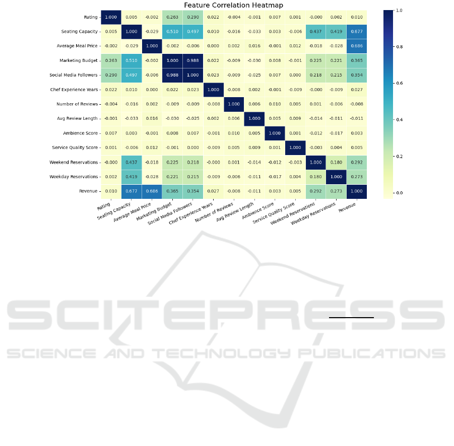
Figure 1: The correlation matrix.

revenue do not mean that they are completely useless,

as the correlation matrix cannot account for the non-

linear relationship. Therefore, this paper will not

simply use the correlation matrix to select the

correlated features.

3.2 Modelling

To fit the model, the first thing to do is calculate the

correlation p-value for each of the numerical

variables, then choose the useful variables. Then the

multiple linear regression model and random forest

model will be built separately.

3.2.1 Correlation P-value

Before calculating the correlation p-value of the

numerical variables, it is tested whether the feature in

question can be seen as Gaussian. This is done by

applying the Shapiro-Wilk test to each of the

numerical variables. If a feature could be seen as

Gaussian, the Pearson test would be applied to

calculate the p-value of the correlation between that

feature and the target variable. If not, the Spearman

test would be used to obtain the correlation p-value

(Bishara & Hittner, 2012).

3.2.2 Shapiro-Wilk Test

Shapiro-Wilk test is widely used to test whether the

sample can be regarded as normally distributed

(Razali, & Wah 2011). Here Shapiro-Wilk test will be

applied to each numerical variable to see if they can

be seen as a Gaussian. To achieve it, the null

hypothesis would be “The feature can be seen as a

Gaussian”, then (1) are going to be used to calculate

the result:

𝑊 =

(

∑







()

)







∑

(





)







(1)

To be specific, in the formula, 𝑥

(



)

is the ith data

after arranging the sample in the ascending order. x ̅

is the mean value of the sample. a_i is the weight

coefficient calculated from the mean and covariance

matrix of the expected normal distribution. Moreover,

as the Shapiro-Wilk test is suitable for use with

relatively small sample sizes, the first 5,000 entries of

each feature to increase the confidence in the results.

After implementing Shapiro-Wilk test, the p-

value of the test is obtained. If the p-value is larger

than the significance level, the null hypothesis will be

accepted, and the feature will be seen as a Gaussian.

3.2.3 Pearson Test

If feature is accepted as a Gaussian, Next step is to

use the Pearson test to test whether the feature is

relevant to the target variable. Here the null

hypothesis would be “the feature is not correlated to

the target variable”, which means here only when the

correlation p-value is smaller than the significance

level it will be picked as the useful feature. To get the

correlation p-value, the first thing to calculate is the

Pearson correlation coefficient(r).

ECAI 2024 - International Conference on E-commerce and Artiﬁcial Intelligence

302

𝑟 =

∑

(𝑥



−𝑥

)(𝑦



−𝑦)







∑

(𝑥



−𝑥

)







∑

(𝑦



−𝑦)







(2)

Here x represent for the feature and y is the target

variable. After calculating, it will be translated into a

t statistic. To be specific:

𝑡 = 𝑟









, where n is the

number of samples. Next is to calculate the

correlation p-value based on the distribution of t-

statistic

3.2.4 Spearman Test

The Spearman test would be used when the feature

cannot be seen as a Gaussian. The basic step is similar

to the Pearson test, and to get the correlation

coefficient, the following formula would be used.

𝜌 =1−

∑

𝑑





𝑛(𝑛



−1)

(3)

Here, 𝑑



is the rank difference of each pair of

observations of two variables, and the calculation

formula is (𝑑



= 𝑅(𝑥



) −𝑅(𝑦



)), where ( R(𝑥



) ) and

( R(𝑦



) ) are the rank of (𝑥



) and (𝑦



). n is the number

of samples. To get the rank, the observed value of

each variable is sorted from small to large and assign

the corresponding rank. For example, the smallest

value has rank 1, the second smallest value has rank

2, and so on. If there are identical values, the average

rank is used.

After calculating the 𝜌, the correlation p-value

would be calculated.

3.2.5 Useful Features

After implementing these three tests, the following

result is obtained (See Table 3). From the result, it can

be seen that none of the numerical variables can be

seen as a Gaussian, so the Spearman test is just

applied to each of them. After calculating the

correlation p-value, the features that the correlation p-

value is smaller than 0.05 are chosen as useful

features.

Table 3: The p-value of numerical variables.

Column Normality

p-value

Correlation

p-value

Method

Rating 2.05*10

-45

7.27*10

-1

Spearman

Seating

Capacity

4.52*10

-44

Spearman

Average Meal

Price

3.68*10

-49

Spearman

Marketing

Budget

5.76*10

-57

4.75*10

-200

Spearman

Social Media

Followers

1.16*10

-54

6.88*10

-187

Spearman

Chef

Experience

Years

1.00*10

-47

1.44*10

-3

Spearman

Number of

Reviews

8.35*10

-46

3.17*10

-1

Spearman

Avg Review

Length

8.03*10

-45

2.53*10

-1

Spearman

Ambience

Score

1.61*10-

5.12*10

-1

Spearman

Service

Quality Score

5.49*10

-45

5.50*10

-1

Spearman

Weekend

Reservations

2.36*10

-44

2.94*10

-153

Spearman

Weekday

Reservations

6.20*10

-45

1.62*10

-120

Spearman

By the table, finally the features that the

correlation p-value are smaller than 0.05 are chosen,

that are: Seating Capacity, Average Meal Price,

Marketing Budget, Social Media Followers,

Weekend Reservations, Weekday Reservations.

3.2.6 Multiple Linear Regression

The first method to be used is Multiple Linear

Regression. Multiple linear regression (MLR) is

effective for prediction because it can consider

multiple independent variables simultaneously and

capture the combined influence of these factors on the

dependent variable. By assuming a linear

relationship, MLR simplifies the model, making it

computationally efficient while still providing

accurate predictions. In addition, MLR's ability to

quantify the contribution of each predictor helps to

understand the impact of different variables, leading

to more reliable and interpretable predictions.

(Breiman, & Friedman, 1997)

To build the model, the whole dataset would be

spilled into train set and test set, where 80% of the

whole dataset as train set, the rest as train set. To build

the model, the below formula would be used:

𝑦 = 𝛽



+ 𝛽



𝑥



+ 𝛽



𝑥



+ 𝛽



𝑥



+ ⋯+ 𝛽



𝑥



(4)

Here y is the predicted annual revenue of

restaurant, 𝑥



represents the ith feature. 𝛽



is the

coefficient of ith feature.

3.2.7 Random Forest Model

The second method to be used would be a random

forest model (See Figure 2). Random forests are well

Restaurant Revenue Prediction Using Machine Learning: A Comparative Study of Multiple Linear Regression and Random Forest Models

303

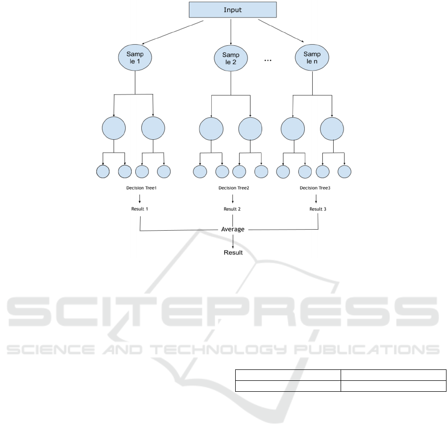
Figure 2: Random Forest Flowchart.

suited for prediction due to their ability to handle

large datasets with numerous features while reducing

the possibility of overfitting (Zhang, Zimmerman,

Nettleton, & Nordman, 2020). By constructing

multiple decision trees and averaging their

predictions, random forests improve model accuracy

and robustness. Meanwhile, random forest models

can deal with these features that may have a non-

linear relationship, making them versatile for

different types of data. In addition, Random Forests

are less sensitive to noisy data and can provide feature

importance metrics, helping to identify the most

influential predictors in the data set.

This diagram above shows how Random Forest

works. After inputting the data, a random portion of

the sample is extracted as a unit, and several such

units form several decision trees. The average of the

predictions of these decision trees is the result of the

prediction.

4 RESULTS

4.1 Multiple Linear Regression

To get the result, the whole dataset is spilled into

training set and test set, where 80% of the whole

dataset is used as training set and the rest is the test

set. Before training the model, the StandardSclar in

Sklearn would be used. Preprocessing to standardise

the features. The mean square error and R2 score are

used to show the error and fitting performance of the

model, and the MSE and R2 score are calculated

based on the test set (See Table 4).

Table 4: The MSE and R2score of MLR.

MSE

3.19*10

0.956

The predicted value in test set is shown to have a

clear comparison between them and the true value of

the restaurant's annual revenue (See Figure 3).

From the result, it can be observed that the fitting

performance of MLR is relatively good since its

R2score achieves 0.955, which is quite high.

However, the Mean Square Error is quite high, which

means it is still needed to improve the model

performance.

4.2 Random Forest

After splitting the whole dataset as above, and after

standardising the features, the model is trained. To

show the goodness of fit and error of the model, the

predicted value is compared to the true value in the

same way as for MLR (See Figure 4). From the result

it can be observed that the R2 score of Random Forest

method is 0.999, which implies the fitting

ECAI 2024 - International Conference on E-commerce and Artiﬁcial Intelligence

304

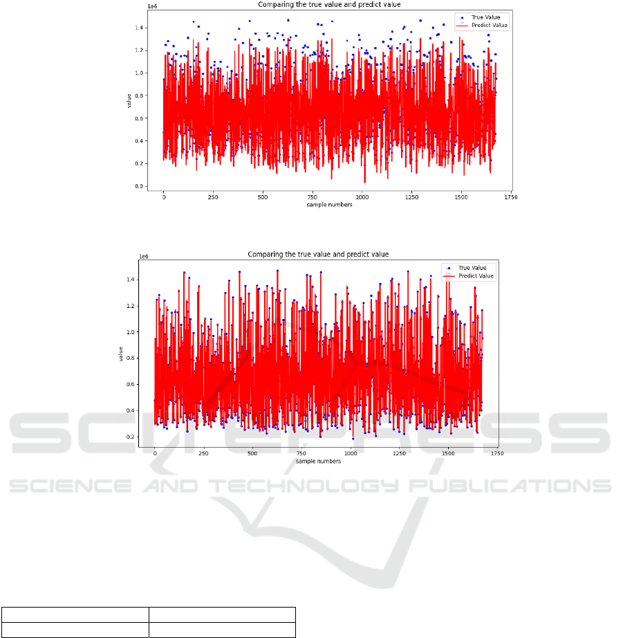
Figure 3: The predict result from MLR.

Figure 4: The predict result from MLR.

performance of this method is quite good since it is

very close to 1. Meanwhile, the MSE of it is also

relatively small, supporting the result of Random

Forest is good (See Table 5).

Table 5: THE MSE and R2score of Random Forest.

MSE

6.29*10

0.999

4.3 Comparison of MLR and RF

Comparing these two results, the fitting performance

of the Random Forest is indeed better than the simple

regression model, as not only is its R2 score greater

than that of the MLR, but the MSE is also relatively

smaller than that of the MLR. There are several

reasons for this, for example, the MLR can only

handle the variables that have a linear relationship

between them. However, by using the Random Forest

method, the variables that have a non-linear

relationship between them can be handled.

Meanwhile, as the results show, by selecting the

useful variables by correlation p-value, the models

are more reliable due to the high R2score of them.

5 CONCLUSION AND

LIMITATIONS

In general, this study has successfully applied

Multiple Linear Regression (MLR) and Random

Forest (RF) to predict restaurant revenue. By focusing

on the numerical variables, models that efficiently

captured the relationships between key features and

revenue outcomes are able to be built. The method of

simplifying the dataset by excluding non-numeric

variables due to their near-identical distribution has

successfully reduced model complexity and helps to

focus on the most relevant predictors. In addition, by

calculating and analysing the correlation p-values, it

is able to refine the model by selecting only the most

statistically significant variables, resulting in

improved model accuracy and fitting performance.

Restaurant Revenue Prediction Using Machine Learning: A Comparative Study of Multiple Linear Regression and Random Forest Models

305

However, the study still has some limitations. For

instance, the exclusion of non-numerical variables,

may have overlooked important qualitative factors

such as location while it indeed can simplify the

model. Meanwhile, the reliance on p-values for

feature selection, while effective in improving model

accuracy, can sometimes lead to the exclusion of

variables that may have practical significance but do

not meet the strict statistical criteria. These

limitations suggest that while the current model has

well-fitting performance, there is potential for further

improvement by incorporating qualitative variables

and exploring alternative methods of feature

selection.

REFERENCES

Bera, S. (2021). An application of operational analytics: for

predicting sales revenue of restaurant. Machine

learning algorithms for industrial applications, 209-

235.

Bishara, A. J., & Hittner, J. B. (2012). Testing the

significance of a correlation with nonnormal data:

comparison of Pearson, Spearman, transformation, and

resampling approaches. Psychological methods, 17(3),

399.

Breiman, L., & Friedman, J. H. (1997). Predicting

multivariate responses in multiple linear regression.

Journal of the Royal Statistical Society Series B:

Statistical Methodology, 59(1), 3-54.

Guyon, I., & Elisseeff, A. (2003). An introduction to

variable and feature selection. Journal of machine

learning research, 3, 1157-1182.

Gogolev, S., & Ozhegov, E. M. (2019). Comparison of

machine learning algorithms in restaurant revenue

prediction. In International Conference on Analysis of

Images, Social Networks and Texts (pp. 27-36). Cham:

Springer International Publishing.

Parh, M. Y. A., Sumy, M. S. A., & Soni, M. S. M.

Restaurant Revenue Prediction Applying Supervised

Learning Methods. Retrieved from

https://www.researchgate.net/profile/Most-

Soni/publication/371756285_Restaurant_Revenue_Pre

diction_Applying_Supervised_Learning_Methods/link

s/6493957995bbbe0c6edf2cd0/Restaurant-Revenue-

Prediction-Applying-Supervised-Learning-

Methods.pdf.

Razali, N. M., & Wah, Y. B. (2011). Power comparisons of

shapiro-wilk, kolmogorov-smirnov, lilliefors and

anderson-darling tests. Journal of statistical modeling

and analytics, 2(1), 21-33.

Siddamsetty, S., Vangala, R. R., Reddy, L., & Vattipally, P.

R. (2021). Restaurant Revenue Prediction using

Machine Learning. International Research Journal of

Engineering and Technology (IRJET) e-ISSN, 2395-

0056.

Steiger, J. H. (1980). Tests for comparing elements of a

correlation matrix. Psychological bulletin, 87(2), 245.

Zhang, H., Zimmerman, J., Nettleton, D., & Nordman, D.

J. (2020). Random forest prediction intervals. The

American Statistician.

ECAI 2024 - International Conference on E-commerce and Artiﬁcial Intelligence

306