A Comparative Analysis of Bitcoin Price Forecasting Approaches

Using Machine Learning Techniques

Boyin Deng

Department of Natural Science, University of Manchester, Manchester, U.K.

Keywords: Bitcoin, Machine Learning.

Abstract: One way to pay for products and services online is with cryptocurrency. Price swings in the cryptocurrency

market may have macroeconomic repercussions because they are a component of the global economic system.

Since Bitcoin is the most recognizable cryptocurrency, predicting its price has gained much attention in the

current financial community. This article compares the impacts of three models — linear regression (LR),

support vector machines (SVM), and long short-term memory (LSTM) — and uses stacked models to conduct

additional research on the price of Bitcoin using machine learning techniques. The experimental results

indicate that the LSTM model effectively captures Bitcoin price volatility, resulting in more accurate

predictions. At the same time, the LR and SVM models are more straightforward in predicting the price. The

stacked model captures the market trend more comprehensively and provides a more valuable reference for

investors. By effectively predicting the price of Bitcoin, this study not only demonstrates the potential of

different machine learning models to be applied in the financial field but also provides investors and

researchers with new perspectives to help them better understand and cope with the complexity and

uncertainty of the cryptocurrency market.

1 INTRODUCTION

Cryptocurrency is a type of money that only exists

digitally or virtually, yet it still uses cryptographic

methods to protect transactions. Cryptographic code

contains pre-established protocols that must be

followed in order to create new units of currency.

Cryptocurrencies are not produced by a central

authority or regulator. A computer programmer by

the name of Satoshi Nakamoto presented the concept

of a virtual currency with guidelines for issue,

distribution, and security measures on his website in

November 2008. Satoshi Nakamoto invented the first

Bitcoin in January 2009. The first-ever Bitcoin

transaction happened in January 2009, the same year

that Satoshi Nakamoto invented the first version of

the cryptocurrency (Cai, 2017).

From the micro level, exploring the price

mechanism of Bitcoin can establish a reasonable

understanding for people who want to invest in

Bitcoin, help them to have a more reasonable estimate

of its price when investing in Bitcoin in the future,

and provide help and support for the choice of

https://orcid.org/0009-0000-3646-4972

investors. From the macro level, implementing digital

currency is an inevitable trend. Since all countries are

developing digital currencies, the study of Bitcoin,

the pioneer of digital cryptocurrency, is conducive to

the development of digital currencies in various

countries, which is of practical significance for the

research development and promotion of digital

currencies and is also of great significance for the

benign development of the financial system as a

whole.

On the other hand, regarding Bitcoin price

prediction methods, Poyser (2018) analyzed and

predicted the price dynamics of cryptocurrencies to

some extent by applying some of these methods from

most traditional financial markets. Several

researchers have ventured into utilizing econometric

methodologies, inclusive of Vector Autoregression

(VAR), Ordinary Least Squares (OLS), and Quartile

Regression (QR), to meticulously examine the

intricate interplay between economic and

technological factors that shape the dynamics of the

Bitcoin exchange rate. Furthermore, the price and

volatility of Bitcoin were predicted by Katsiampa

Deng, B.

A Comparative Analysis of Bitcoin Price Forecasting Approaches Using Machine Learning Techniques.

DOI: 10.5220/0013214500004568

In Proceedings of the 1st International Conference on E-commerce and Artiﬁcial Intelligence (ECAI 2024), pages 263-268

ISBN: 978-989-758-726-9

263

(2017), Selin (2020), and Duan et al. (2020) using

conventional time series forecasting techniques such

as univariate autoregression (AR), univariate moving

average (MA), simple exponential smoothing (SES),

and autoregressive integrated moving average

(ARIMA) (Jing, 2021). However, Cheng et al. (2010)

argued that these methods are not very practical for

this forecasting task due to the lack of seasonality and

high volatility of the cryptocurrency market and the

use of statistical models, which require that the

models only deal with linear problems and that the

variables must follow a normal distribution (Jing,

2021). Both the forecasting of digital currencies and

the challenge of asset price and return forecasting

have seen the application of machine learning

techniques in recent years. Machine learning

techniques have been applied successfully to stock

market forecasting by incorporating nonlinear

features into the forecasting model to deal with non-

stationary financial time series; the findings have

shown that the method is more effective for

predicting (Yuan et al., 2016). Dinh et al. (2018)

predicted the price of Bitcoin using recurrent neural

networks and long short-term memory (LSTM). The

results demonstrated that the machine learning

approach, with its advanced temporal properties,

could produce better predictions than the

conventional multi-layer perceptron (MLP) (Jiang,

2020).

This paper delves into Bitcoin prediction utilizing

a machine-learning framework. Its objective is to

scrutinize the strengths and weaknesses of diverse

machine learning models in forecasting Bitcoin prices

and conduct a comparative analysis as a pivotal

reference for financial scientists seeking to anticipate

Bitcoin's future price movements.

2 DATASETS AND METHODS

2.1 Datasets

The data used in this study is taken from Kaggle’s

official website, and the dataset is about the Bitcoin

price from 2014.09.17 to 2024.07.07 with the daily

opening and closing prices. This article first converts

the Date column of the data to a date format, sorts by

date, and then normalizes the Close column to

between [0,1]. Finally, this paper defines the

create_dataset function to create a time series dataset,

divides the dataset into a training set (80%) and a test

set (20%), and then adjusts the time step to adjust the

data to the 3D format required by the LSTM model.

2.2 Models

LR serves as a fundamental model for predicting

continuous-valued target variables. It postulates a

direct, linear correlation between the input features

and the output targets. By minimizing the mean

square error (MSE) between the predicted and

observed values, the linear regression (LR) model

identifies the optimal line that best fits the data. On

specific model parameters, the fit_intercept of the

model is set to True; that is, the model calculates the

intercept term of the model. The model's normalized

setting is set to False, which means that the model

does not normalize the regression variables until

fitted.

LSTM is a recurrent neural network (RNN)

capable of processing and predicting long-term

dependency problems in time series data. The LSTM

can handle the dependencies of data over a longer

time frame through its internal memory unit. The

number of LSTM layers used in this article is two; in

the first layer of the LSTM, the number of LSTM

cells (is 50). return_sequences is True. The

input_shape is the shape of the input data, set to (30,

1); that is, the time step is 30, and the number of

features is 1. In the second layer of the model, the

return_sequences is set to False, indicating that only

the output of the last time step is returned. Dense (1)

is a fully connected layer to output prediction results.

Support vector machines (SVM) is a classical

supervised learning algorithm for binary and multi-

classification problems. The basic idea is to draw an

optimal hyperplane in the feature space for

classification. Support vector regression (SVR) is

nothing but the type of SVM for the regression model.

In a nutshell, SVR tries to fit the error within a certain

threshold because it optimizes for finding a

hyperplane with as many training samples within this

range of errors from itself, using regularization

parameters that help put constraints on model

complexity. Regarding specific model parameters,

the kernel of the model is set to radial basis function

(RBF). The regularization parameter has been tuned

to 100 to balance the model's complexity and training

error. This adjustment helps prevent overfitting by

penalizing complex models. Additionally, the kernel

coefficient has been set at 0.1, a value that dictates the

extent to which individual training samples influence

the shape of the decision boundary. Furthermore, an

epsilon tube of 0.1 has been established, ensuring that

the model's predictions falling within this margin of

error are not penalized. This approach allows for

flexibility in prediction accuracy, accommodating a

range of minor deviations from the exact target value.

ECAI 2024 - International Conference on E-commerce and Artiﬁcial Intelligence

264

2.3 Stacking Model

Stacking is an ensemble learning technique that

enhances the accuracy of the overall predictions by

combining the predictions of several underlying

models. The model has two layers of stacking: one is

a different base learner, and the second is a meta-

learner for combining base learners. In this study, the

prediction results of different basic models are

obtained separately, and then these results are

combined into a new feature matrix. Each column of

the new feature matrix represents the prediction of a

base model. Finally, the stacked feature matrix

train_predict_stacked and test_predict_stacked is

passed to the meta_model for final prediction.

3 RESULTS AND DISCUSSION

3.1 Model Performance Indicators

The evaluation metrics used in this model of the paper

are MSE, mean absolute error (MAE), and coefficient

of determination (R



). Mean Squared Error (MSE):

As defined in equation (1). It computes the overall

sample error by squaring the error between the

predicted and actual values for all the samples. A

lower MSE indicates that the model predictions are

more accurate (less distance between predicted and

actual). Equation (2) outlines the computation of

MAE, and his calculation involves summing up the

absolute differences between the predicted and actual

values for each sample, subsequently dividing the

result by the total number of samples 𝑛 . MAE

exhibits reduced sensitivity to outliers due to its

reliance on absolute values rather than squared

deviations, making it a robust indicator. Moreover,

the coefficient of determination (R



) described by

equation (3) ranges between 0 and 1, with values near

1 indicating a better model fit. This measures how

well the model explains the variation in the data –

larger values indicate better explanatory power.

𝑛represents the total number of samples and 𝑦



denotes an individual sample within the dataset.

MSE =

𝑛





𝑦



−𝑦















MAE =





−y













∑

y



−y







∑



−y









3.2 Experimental Results

Table 1 shows the experimental results in this paper,

with each data point taken to 9 decimal places.

Table 1: Training and test set performance metrics.

MSE MAE



Train

0.005163576 0.042646489 0.900274667

LR Test

0.018228223 0.121187024 0.65930544

LSTM

Train

0.000143822 0.007205582 0.997222332

LSTM

Test

0.000251676 0.010949048 0.995296045

SVM

Train

0.004755175 0.062103502 0.908162208

SVM

Test

0.001276630 0.025976097 0.976139156

Stacking

Model

Train

0.000134628 0.006685161 0.997399897

Stacking

model

Test

0.000229660 0.009578838 0.995707537

The table reveals that the LR model demonstrates

a lower MSE on the training set, indicating a minimal

prediction error and a narrow margin of difference

between the model's predicted outcomes and the

actual values. Further, the model's MAE is also kept

at a shallow level, which is relatively small in the

normalized data. The coefficient of determination



) indicates that the model can account for variance

in 90% of the training data, indicating that the LR

model fits very well on the training set, capturing the

linear trend of most of the data. Although the test

performance of MSE and MAE increased compared

with the training set, they were still within a

reasonable range, indicating that the model performed

reasonably on the test partition; the low R



on the test

partition indicates that there may be nonlinear solid

relationships in the data, and LR does not handle

these complex features well. The second is the LSTM

model, which can be seen from its training

performance, with low MSE and MAE, indicating

that LSTM can also make better predictions on the

training set. The coefficient of determination R



higher than that of LR, which may mean that LSTM

has a slight advantage in capturing nonlinear

relationships in the data. While the stacked model

excels within the training environment, its

performance trends in the test set mirror those

observed during training, attesting to its consistency.

Notably, despite a slight, statistically insignificant

increase in MSE and MAE for the LSTM model in

A Comparative Analysis of Bitcoin Price Forecasting Approaches Using Machine Learning Techniques

265

the test set compared to the training set, its R



score

remains commendable, underlining its reliable

performance in both scenarios. Conversely, the SVM

model's training performance reveals significantly

higher MSE and MAE values than the LSTM,

signifying a lesser fitting proficiency. Despite this,

the SVM's R



coefficient, albeit lower than the

LSTM's, surpasses 0.90, evidencing a decent

predictive capacity within the training domain.

Interestingly, when assessed on the test set, the SVM

exhibits a comparatively low MSE, hinting at its

inherent capability to mitigate overfitting. Though its

MAE remains elevated yet reduced from the training

phase, this reduction points towards an improved

generalization capability of the SVR in the test

environment. Furthermore, an R



score nearing 0.98

underscores the SVM's impressive prediction

accuracy within the test set. Ultimately, by

amalgamating the strengths of three distinct models,

the stacking model emerges victorious, surpassing its

components in training and testing. This integrated

approach harnesses the best attributes of each model,

resulting in enhanced overall performance across the

board.

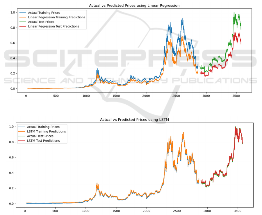
As evident from Figures 1, 2, 3, and 4, the LR

model employs a relatively straightforward and direct

approach to prediction, simplifying estimating

outcomes. Although some trends are captured in the

training data, the performance in the test data part is

significantly worse than that of other models. The red

line forecasts the price (green) and a substantial

deviation due to the limitations of linear models

working with non-linear time-series datasets. In the

initial stages of the training set, the SVM model

exhibited prediction results that deviated significantly

from the actual prices. However, as the training

Figure 1: LR prediction and actual values (Photo/Picture credit: Original).

Figure 2: LSTM prediction and actual values (Photo/Picture credit: Original).

ECAI 2024 - International Conference on E-commerce and Artiﬁcial Intelligence

266

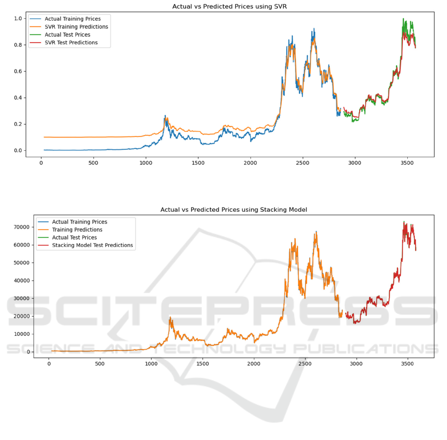
Figure 3: SVM prediction and actual values (Photo/Picture credit: Original).

Figure 4: Stacking Model prediction and actual value (Photo/Picture credit: Original).

progressed, the predictions gradually converged with

the actual values, ultimately demonstrating a high

level of agreement and consistency in the training

outcomes. However, there was a significant

difference in some turning points, indicating it was

not very sensitive to volatility. The predicted price of

the ensemble model is in good agreement with the

actual price, especially in the test data section, where

the model successfully captures the trend. The slight

deviation between the test price and the red forecast

line indicates that the model fits very well.

Similarly, the predictions of the LSTM model

closely follow the actual price. Compared to the

stacking model, the deviation is slightly larger at

some points, but the overall prediction is still entirely

accurate. LSTM excels at capturing long-term

dependencies in time series, which is reflected in the

accuracy of the graphs.

In summary, the stacked model outperforms both

LSTM and SVM, with LSTM ranking second and

SVM performing inferiorly to the first two in the

training set. Still, the performance in the test set is

acceptable, and the prediction results align with the

actual price. At the same time, LR cannot cope with

complex and nonlinear data. Therefore, when

predicting the price of Bitcoin, due to its intense

volatility, models with nonlinear solid data

processing capabilities, such as LSTM, will perform

better than other models. In contrast, stacking models

can combine the advantages of multiple models to

make the prediction results more realistic.

A Comparative Analysis of Bitcoin Price Forecasting Approaches Using Machine Learning Techniques

267

4 CONCLUSIONS

Bitcoin is the origin of modern cryptocurrency, and

studying its price movements can analyze the

market's optimism about cryptocurrencies, so its

research is one of the most popular topics of

discussion among financiers. This study compares the

predictive abilities of LR, SVM, LSTM, and stacking

models on Bitcoin price movements. Through

analysis, this paper finds that different models have

advantages and disadvantages in capturing price

trends. The stacked model can combine the

advantages of different models to a certain extent so

that the prediction results are closer to reality. Despite

this, there are some limitations to this study. First, the

model's prediction outcomes rely heavily on the input

data's caliber and feature selection. In practical

applications, the noise and absence of data may affect

the model's performance. In addition, tuning the

model's hyperparameters and selecting the training

set may also significantly impact the final prediction

results. Future research endeavors can delve deeper

into exploring the vast potential of more intricate,

deep learning architectures and hybrid models,

particularly in tackling high-dimensional and

inherently nonlinear datasets, thereby enhancing their

applicability and effectiveness. The experiment can

also introduce external variables, such as

macroeconomic indicators and market sentiment, to

improve the model's generalization ability and

forecasting accuracy. Through these efforts, investors

and financial institutions can be provided with more

accurate price forecasts, helping people make more

informed decisions in an uncertain market

environment. This will not only help improve

financial market stability but also promote the further

development of quantitative investment strategies.

REFERENCES

Cai, K., 2017. Can Bitcoin Be Invested In? China Securities

& Futures, 5.

Cheng, C. H., Chen, T. L., Wei, L. Y., 2010. A hybrid

model based on rough sets theory and genetic

algorithms for stock price forecasting. Information

Sciences, 180(9), 1610-1629.

Dinh, T. A., Kwon, Y. K., 2018. Using neural networks, an

empirical study on modelling parameters and trading

volume-based features in daily stock trading.

Informatics, 5(3), 542–547.

Duan, J., Zhang, C., Gong, Y., Brown, S., Li, Z., 2020. A

content-analysis based literature review in blockchain

adoption within food supply chain. International

Journal of Environmental Research and Public Health,

17(5), 1784.

Katsiampa, P., 2017. Volatility estimation for Bitcoin: A

comparison of GARCH models. Economics Letters,

158(9), 3-6.

Jiang, X. X., 2020. Bitcoin price prediction based on deep

learning methods. Journal of Mathematical Finance,

10(1), 666–674.

Jing, P. F., 2021. A comparative study on Bitcoin price

prediction based on multiple models (Master's thesis,

Shanxi University).

Poyser, O., 2018. Exploring the dynamics of Bitcoin’s

price: A Bayesian structural time series

approach. Journal Name, 10(1), 121–129. Springer

International Publishing.

Selin, O. S., 2020. Dynamic connectedness between

Bitcoin, Gold, and Crude Oil Volatilities and

Returns. Journal of Risk and Financial Management,

13(11), 127–136.

Yuan, W., Chin, K. S., Hua, M., et al., 2016. Shape

classification of wear particles by image boundary

analysis using machine learning algorithms.

Mechanical Systems and Signal Processing, 14(5), 72-

73.

ECAI 2024 - International Conference on E-commerce and Artiﬁcial Intelligence

268