Prediction of Daily Lognormal Returns for Bitcoin Based on

LightGBM

Jiaxing Wei

School of Data Science, The Chinese University of Hongkong (Shenzhen), Shenzhen, China

Keywords: Bitcoin, Blockchain, LSTM, CNN, LightGBM.

Abstract: With rapid development in Blockchain technologies, the security of cryptocurrencies like Bitcoin has been

significantly improved. However, as the cryptocurrency with the largest traded volume per day, Bitcoin

continuous to expose to volatile risk due to its intrinsic attributions, including non-supervisory and all-weather.

This research utilizes neural network and tree-based models to predict the short-term future returns of Bitcoin.

The Neural-Network-based models like Long-Short Term Memory (LSTM) and Transformer outperform with

statistical significance. By introducing L2-regularzation, the research discovers an available approach to

alleviate the short-term volatile risk for investors by proposing an embedding model to predict rapid changes

from future returns. While leverages a R-squared that outperform the benchmark by 11%, the embedding

model is verified to maintain efficiency with an enhanced convergence rate. The research analyses 4

commonly used Machine Learning models in financial time-series prediction and compares their

performances with the calibrated embedding model. By contrasting the advantages and corresponding

shortcomings, this research fills the gap in offering suggestions for investors to engage non-supervised market

to decrease exposures in volatile risk.

1 INTRODUCTION

As the first appeared cryptocurrency, Bitcoin (BTC)

was introduced to the world in 2009 by an entity

called Satoshi Nakamoto. Such kind of

cryptocurrencies are runned by the blockchain.

Gorkhali defines blockchain as a kind of distributed

system, which consists of several blocks and

corresponding chains that connect them (Gorkhali,

2020). The information of transaction is stored in

each separated block and the issue of Bitcoin is

conducted by specified protocals (Dinh, 2018).

Blockchain is regraded as the fundement of the new

format of transaction. For the sake of the utilization

of decentralized database to build trust between the

buyer and the seller, without any engagement of the

third party such as conventional exchanges and banks

(Madey, 2017). Kang points out that decentralized

system reduces transaction fees, and provides

anonymity (Kang, 2022).

Madey also indicates such attributions promoted

cryptocurrencies like Bitcoin to expand in a rapid way

and became popular for anonymity within a few years

https://orcid.org/0009-0007-4835-259X

since they had been launched. Simultaneously, the

dramatic increment of Bitcoin’s market capitalization

provided enormous liquidity that supported various of

trading strategies (Madey, 2017). The deep reason for

such increment could be traced back to the fair access

of the cryptocurrency trading market. Like what

D’Aliessi have claimed, the blockchain allows

investors without sophisticated monetary systems to

engage this world-wide market with tremendous

efficiency (D’Aliessi, 2016). However, Farrel

mentions the profits and losses are potentially

originated from the high volatility in cryptocurrencies

(Farrel, 2013). This phenomenon is sufficient to

reveal that there exist potential risks in aspect of the

dramatic price movement. During the early stage of

cryptocurrencies such as Bitcoin, main threats for

holders of these new-born currencies consists of

address attacking (Beikverdi, 2015), double spending

risk (Auer, 2021), and the exposure on volatile

currency (Madey, 2017). Madey addresses that the

blockchain utilizes cryptography function to obtain

immutability and accelerates transaction information

among engagers in the market to eventually eliminate

154

Wei, J.

Prediction of Daily Lognormal Returns for Bitcoin Based on LightGBM.

DOI: 10.5220/0013208400004568

In Proceedings of the 1st International Conference on E-commerce and Artiﬁcial Intelligence (ECAI 2024), pages 154-163

ISBN: 978-989-758-726-9

the double spending risk (Madey, 2017). To prevent

hackings towards ledgers that result in account loss,

the blockchain technology proposed a multi-node-

distribution of ledgers, which hinders such attacking

(D’Aliessi, 2016). Yet Bitcoin remains to be volatile

since small and continous transactions contribute a

large portion to the rapid movement in price (Madey,

2017).

On top of the issue, methodlogies for prediction

are proposed to address the problem. The very first

research concentrates on using Ordinary Least Square

(OLS) regression to fit the future returns of Bitcoin

and other cryptocurrencies. Even OLS is capable in

fitting linear relationship between the label and

independent variables, this method fails to capture

complex non-linear patterns between data (Kar, 2023).

Lahmiri et al. are the scholars first to implement Deep

Neural Network (DNN) on prediction tasks (Lahmiri

et al., 2019). The team proposed a variation of DNN

named Long-Short-Term Memory (LSTM) to

forecast Bitcoin prices (Uras, 2020). Based on Uras’s

research (Uras, 2020), Livieris et al. embedds

Convolution Neural Network (CNN) into the

pipepline to enhance the accuracy (Livieris et al.,

2021). CNN has showcased the utility of skip

connections in time-series data. By spilting the

original input matrix into smaller feature maps, CNN

generates enourmous output layers that regarded as

non-linear explantory variables (Kar, 2023). Another

approach for forecasting is to summarize different

kinds of price movement of Bitcoin and utilize the

historical trends to predict the future returns. The

remarkable investigation of others proposes a new

tree-based pipeline named Light Gradient Boosting

Method (Light GBM) for solving regression

problems with decision trees (Alabdullah, 2022).

Jiang proofs that Light GBM is more effective in

handling large scale data compared with LSTM and

CNN (Jiang, 2017). It also proposes another effiective

method called Transformer with the ability to access

significant pattern within the input time-series data on

the predcition task. The innovation achieves great

improvement in both robustness and accuracy

compared with OLS.

This research aims to evalutate the performance

of popular machine learning algorithms on the

prediction of Bitcoin’s future returns. The second part

of the article introduces all components of research

data and fundemental features sythesized from them.

In addition, corresponding methods for data cleaning

and identification of the predictive label are included.

OLS is set as the benchmark of this prediction task.

On top of the benchmark, the research selects LSTM,

CNN, Light GBM and Transformer as component

pipelines and utilizes three different metrics to

evaluate their performance on historical data. Within

the third part, the article mainly focus on the feature

engineering for model training and testing, and

detailed backtest results of each pipeline. This

research proposes a new embedding pipeline on top

of elementary models to evalutate the performance of

popular pipelines in trend. Since cryptocurrencies like

Bitcoin are the last part of the paper offers

suggestions on Bitcoin investment to reduce volatile

risk that is generated from the instrinct properties of

Bitcoin: all-weather, non-supervisory, and

tremendous market trading engagament.

2 DATA AND METHODS

As previous scholars indicate in the work (Kar, 2023),

machine learning algorithms like Convolution Neural

Network (CNN) reveals the non-linear relationship

between explanatory variables and predictive labels

works better than the traditional linear ones like OLS

regarding cryptocurrency price prediction. On top of

existing results, this research is based on the daily

trading data of Bitcoin and tries to solve its research

questions by implementing various machine learning

methods, such as the Long-Short Term Memory

(LSTM), CNN, Light Gradient Boosting Machine

(LGBM), and Transformer. Alabdullah has

showcased the positive effect that the data balance

has on the model performance (Alabdullah, 2022).

Therefore, relatively balanced data will be introduced

to this research to enhance the robustness and

accuracy of the embedding pipeline for final

prediction.

2.1 Dataset

All data used in the research are fetched from Yahoo

Finance, including daily trading Bitcoin from Jan 1

2016 to Aug 9

, 2024. There are 7 columns in the

dataset include the date, prices information such as

open, high, low, close, adjust close and the traded

volume. This research uses 3,144 lines of daily data

in continuous trading dates.

2.2 Dataset Preprocessing

The procedure could be divided into 3 main parts,

including constructing technique indicators via

Python TA-Lib library, normalizing feature dataset,

and identifying predictive label for the prediction task.

Indicators are constructed to describe the behaviour

of Bitcoin’ trading prices and volumes in the past

Prediction of Daily Lognormal Returns for Bitcoin Based on LightGBM

155

period. They can used as metrics to estimate the

previous performance the asset. In addition to

enhance the ability of the proposed pipeline to explain

the returns of Bitcoin utilizing indicators, it is

reasonable to consider of the similar asset that with a

large market capitalization as well, such as the

Ethereum. Therefore, indicators that represent

correlations between Bitcoin and Ethereum are

introduced as parts of the feature map. Relationships

include the time-series correlations of daily returns,

adjusted close prices, and traded volumes that are

calculating by rolling window method. Except for

common statistics, indicators for Bitcoin are listed as

follow:

 Simple Moving Average (SMA): SMA takes

average of the price in past periods to reduce the

volatility of daily price data. It represents the

trend of Bitcoin’s price movement.

 Exponential Moving Average (EMA): EMA

generates weights on each data point to reduce

the delay rate (Tanrikulu, 2024) on top of the

SMA.

 Relative Strength Index (RSI): RSI estimates

the proportion of upward movement during a

period. It is taken as a popular metric for

estimation the short-term trend of price

movement.

 Detrended Price Oscillator (DPO): DPO

estimates the length of price cycles.

 Momentum: The indicator measures the rate of

increment or decrement in the Bitcoin’s price. It

represents the sustainability of price movement.

 Moving Average Convergence Divergence

(MACD): MACD is a variation of the

Momentum indicator that has been widely

applied to predict future trends since Appel

(1971-) created it.

 William’s Variable Accumulation Distribution

(WVAD): WVAD uses the correlation between

the accumulative distribution of adjacent

trading dates to measure the buying and selling

pressure of Bitcoin.

 Time Weighted Average Price (TWAP): TWAP

measures the average price of Bitcoin over some

time periods.

 Volume Weighted Average Price (VWAP):

Similar to TWAP, VWAP gives weights to

prices based on the traded volumes. This

indicator estimates the impact that volumes

have on the price movement.

 Percentage Volume Oscillator (PVO): PVO is

the ratio of the difference between two moving-

average volumes and the larger one. This one

captures the shift in trends of trading volumes.

 Average Directional Index (ADX): ADX is

regarded as a reliable indicator to predict the

strength of a price trend.

 Cumulative Strength Index (CSI): CSI measures

the relative strength of increasing/decreasing

trends of Bitcoin’s price.

All indicator data are reshaped by the time series

normalization to have factor values of range [-1, 1].

To avoid data leakage, the length of the window for

normalizations is equal to the one for calculation of

indicators. Due to the calculation method and the

attribute of original data (price vs volume), there

could exist significant gap between initial factor

values originated from raw data (Tanrikulu, 2024).

This operation creates comparable results to eliminate

potential biases in data during the fitting procedure.

This research implements the Z-score method to

normalize independent variables: (𝑋 represents a time

series data array, 𝜇 is the average of the array and 𝜎

is the corresponding standard deviation)

𝑍 =

()



(1)

Within this research, the log return of Bitcoin at date

T is implemented as the predictive label, which is

formulated as:

𝑟



 



 



– 1 (2)

𝑙𝑜𝑔

(

𝑟



)

= 𝑠𝑖𝑔𝑛

(

𝑟



)

· 𝑙𝑜𝑔𝑎𝑏𝑠

(

𝑟



)

 (3)

With the combination of the sign of the daily return

that calculated by two adjacent adjusted close price

and the absolute value of the return, the research

keeps data of downward shift returns, which prevents

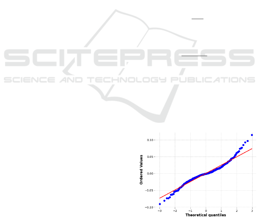
the loss of meaningful information. As shown in

Figure. 1, the closer the predicted value to the red line

(ground truth value), the stronger the normality of the

log-return label.

Figure 1: QQ-plot for log-return of Predicted vs Ground

Truth (Photo/Picture credit: Original).

ECAI 2024 - International Conference on E-commerce and Artiﬁcial Intelligence

156

2.3 Relativity Analysis

In order to reduce the multicollinearity caused by

relatively high correlation between explanatory

variables, the research uses the Spearman’s rank

correlation coefficient to estimate how close each pair

of technique indicators are. For the feature matrix of

n columns 𝑋



=[𝑥



, 𝑥



,...,𝑥



] , each 𝑥



, 𝑖∈[1, 𝑛]

represents values of the corresponding indicators

from time 𝑡



to 𝑡



. Under the OLS framework, if the

label is denoted as 𝑦, the procedure is to solve:

𝑦 = 𝑋



𝛽 + 𝜀 (4)

where 𝜀 is the residual of prediction model, and to

regard the estimated 𝛽 as the ground true coefficient

matrix of each indicator. At the final stage of the

fitting procedure, the matrix will be used to estimate

the future value of labels by inputting new feature

data. If there exists collinearity between any pair of

𝑥



, as Tanrikulu (2024) has published in his work,

there will be a greater bias between the estimated 𝛽

and the ground true one. To prevent being hinder to

enhance the accuracy of prediction from such biases,

the research implements relativity analysis by using

Spearman’s coefficient as the metric to evaluate how

close each indicator is and drop out those with a

correlation higher than a specify threshold.

2.4 Component Models

The LSTM neural network is chained by a row of

LSTM cells. LSTM is capable in predicting the

seasonal trend in time-series data. The advantage of

LSTM, is that the cell can recall memories from any

intervals of the input data, and eventually eliminate

the problem of long-term dependency through

controlling long-term memories by these cells

(Nasirtafreshi, 2022).

CNN extracts high-level vectors from the raw data

in hidden layers and output the processed vectors into

the next level. In contrast of the original k-line data

with low Signal to Noise Ratio (SNR), these vectors

have the relatively higher SNR. CNN also utilizes

pooling layers to shrink the dimensions of input

feature, which can reduce the noise of a time-series

data. According to (), CNN showcases better

performance compared with LSTM or MLP in the

task of Bitcoin trends prediction by reducing the noise

and dimensionality of input financial data.

Light GBM is a various of the Gradient Boosting

Decision Tree that established by Microsoft. It

maintains a balance between performance and

memory-efficiency. Light GBM introduces exclusive

features bundling (EFB) to alleviate overfittings

(Alabdullah, 2022). Still, the most significant

advantage is that Light GBM processes large-scale

data without severe memorial occupation. This

attribute allows investors that own limited

computational source to implement prediction on

future trends of cryptocurrency.

Transformer is a neural network framework that

well known for its capacity in extracting statistical

and non-linear pattern in time-series data. Khaniki

showcases that Transformer leverages the ability to

capture such statistically significant within short

periods by exhibiting promise (Khaniki, 2023).

Utilization of the attention mechanism enhances the

ability for Transformer to adapt to shifts in data

distribution as the training windows change, which

helps the model grasp both long-term and short-term

attributes of Bitcoin prices.

2.5 Evaluation Metrics

In this research, 3 metrics are selected as the criteria

to estimate the performance of each elementary

pipeline and the embedding model from two different

perspectives. At the first stage of evaluation, mean

squared error (MSE) and mean averaged error (MAE)

are served as basins to demonstrate the component

pipeline exhibits lower MSE and MAE to the

benchmark (Khaniki, 2023). The robustness of

prediction methods ensures their durability to adapt to

shifting market conditions. The process turns to the

comparison on R-Squared for revealing accuracy and

effectiveness of each pipeline and the embedding

model. The model with larger R-squared is identified

as the more effective one since the increased R-

squared enhances the statistical significance of the F-

value. Mean-Square Error (MSE) is a metric that

measures the average squared difference between

observation and prediction. The square property

makes it a proper loss function for the evaluation of

the prediction model. MSE is defined as:

𝑀𝑆𝐸 =







(

𝑦



−𝑦



)







(5)

where 𝑦



refers to the ground true value of dataset

contains 𝑛 samples and 𝑦



means the predicted value

generated from the model.

Mean-Absolute Error measures the average

absolute error between predicted values and ground

true values. The linearity of MAE provides less

sensitivity to extreme values in the distribution. The

metric is formulated as:

𝑀𝐴𝐸 =





∑

|𝑦



−𝑦







(6)

𝑅



refers to the proportion of the variance in the

dependent variable that can be explained by the

independent variable. It measures the ability of

explanation from independent variables in the model.

Prediction of Daily Lognormal Returns for Bitcoin Based on LightGBM

157

The value of this indicator domains in [0, 1], with a

better fitness in data as it increases. R-squared is an

efficient metric to estimate the performance across

different predictive models. It can be derived as:



∑

(









)







∑

(







)







(7)

3 RESULTS AND DISCUSSION

3.1 Feature Engineering

The research implements relativity analysis at the

beginning stage of this part. To alleviate the negative

impacts from multicollinearity between independent

variables, relativity analysis is proposed to estimate

the correlation of them. In order to maintain the

explanatory attributes of technique indicators, with

the upper bound threshold of Spearman rank

correlation coefficient to be set as 35%. The remained

feature map consists of 18 different components after

the relativity filtration. For each pair which contains

the same type of features, the same metric is utilized

to estimate the rank of its components. The most

irrelevant one is reserved. The degree of

multicollinearity could be estimated via the Variance

Inflation Factor (VIF). The indicator measures the

increment of variance of the regression model that is

contributed by multicollinearity. Figure. 2& 3 shows

the improvement of the filtration that the degree of

multicollinearity is significantly decreased for each

indicator.

Figure 2: Reserved features after relativity analysis (Photo/Picture credit: Original).

ECAI 2024 - International Conference on E-commerce and Artiﬁcial Intelligence

158

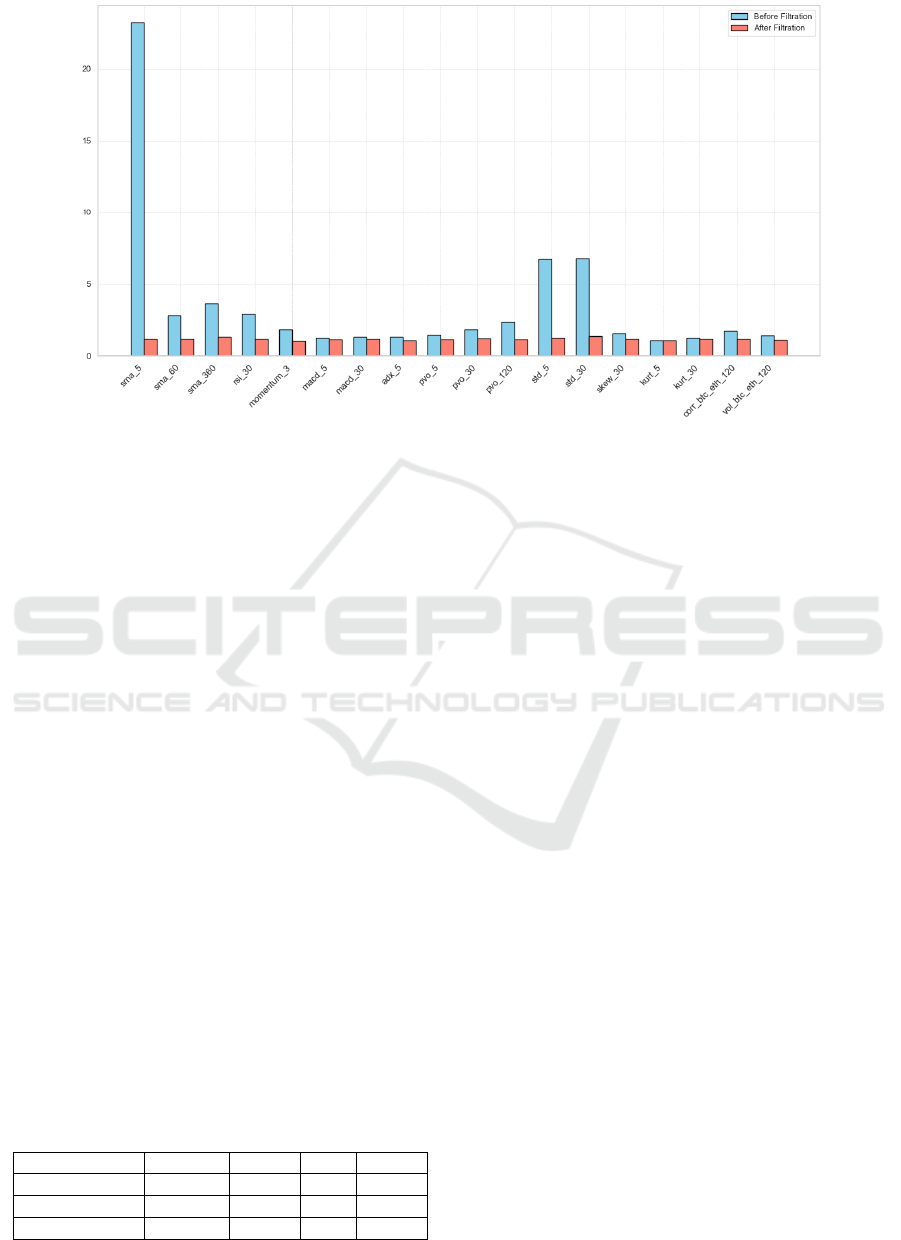
Figure 3: VIF of features Before & After Filtration (Photo/Picture credit: Original).

3.2 Training & Testing Scheme

The training and validation set takes the portion to 80%

while the test set takes the rest of the input data. K-

fold method is implemented to guarantee the

robustness of each prediction. To prevent data leaking,

the time-series data will be transmitted into the model

with a rolling scheme. Specifically, the complete data

will be split into 10 parts with equal lengths, and these

subsets should be further split into training and testing

parts. Therefore, the original data is separated into 10

sub-data to increase the number of training and

testing. The shuffle method is strictly prohibited

during the procedure. The loss function for pipeline,

as this paper has mentioned in section 2.5, will be a

combination of MAE and MSE. OLS is set as the

benchmark of prediction tasks.

Each NN-based model in the research is

constructed by the following structures. This research

implements simple structures to examine the ability

for them to predict future log returns of Bitcoin during

which utilizing shallow layers to extract important

and explanatory features from original indicators.

Here, HL, PL, FC, AF refer to the number of hidden

layers, pooling layers, fully-connected layers, and

activate functions, respectively. The results are

summarized in Table 1.

Table 1: Structure of Neural Network Models.

Model HL PL FC AF

CNN 2 1 1 ReLU

LSTM 3 1 2 ReLU

Transforme

3 N/A 3 ReLU

3.3 Model Performance

The performance of the 4 selected pipeline on the test

set with the 10-folds cross validation is demonstrated

in Table 2. The results are shown in Figure. 4 and

Figure. 5. The R-squared to the benchmark is

significantly low that approaches zero. The result

indicates that if one utilizes the OLS to predict the

future log returns of Bitcoin, the accuracy differs little

to utilizing the mean value of the time-series for the

same task. While utilizing a CNN with relatively

simple structure, the R-squared increases up to 2.95%.

The outcome confirms the inference that CNN are

more capable in capturing non-linear relationship

between technique indicators and the log return of

Bitcoin. As the improved variation of CNN (Uras,

2020) that construct forget layers to drop long-term

memories that may be inefficient within specific

short-term periods, LSTM outperforms CNN in

aspect of the R-squared that high up to 8.4%. On top

of LSTM, Transformer introduces more advanced

encoders to calibrate the ordered input time-series

financial that boosts the R-squared to 10%, which

outperforms the benchmark and even its variations.

The Light GBM, regarded as the simpler one, consists

of less layers for high-dimensional vector processing.

Contrast to the complicated structure of neural

network, Light GBM uses embedding decision trees

to premise the efficiency (Alabdullah, 2022). Yet the

model obtains a R



of 5.97%, which beats the

benchmark without requiring for complex

architecture designs. The research discovers that

comparing with the traditional method that utilizes

Prediction of Daily Lognormal Returns for Bitcoin Based on LightGBM

159

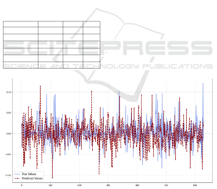
multi-indicators and OLS to fit the future return, the

machine learning pipeline is more capable in such

predictions. Even the single model can boost the

model to a higher R-squared value. The

implementation of machine learning algorithms

enhances the accuracy for investment predictions and

results in a corresponding lower volatile risk.

Specifically, as the outlier among the benchmark and

other pipelines, Transformer and LSTM demonstrate

stronger abilities to confirm and capture the short-

term trend, especially for dramatic jumps. To further

improve the performance, the research proposes a

simple embedding model based on the best performs

pipeline. To reduce outcomes of extreme values, the

L2 regularization is assembled into the Transformer.

With the square loss term, the embedding model tends

to reduce the magnitude in prediction. The

corresponding loss is:

𝐿𝑜𝑠𝑠



= 𝐿𝑜𝑠𝑠



+ 𝜆 |𝜔









(8)

Table 2: Evaluation Statistics over 1,000 epochs.

Model MSE MAE

R²

OLS 0.0012 0.0238 0.0020

CNN 0.0024 0.0313 0.0295

LSTM 0.0006 0.0177 0.0842

Light GBM 0.0010 0.0246 0.0597

Transformer 0.0017 0.0314 0.1004

Transformer-L2 0.0006 0.0175 0.1103

Another important metric to estimate the

performance of pipelines refers to the convergence

rate of them. The rate is calculated by the simple

average of corresponding MAE and MSE for each

epoch within any single subset of input data. During

the training process, as being shown in Figure. 6,

Figure. 7 and Figure. 8, the convergence rate of MAE

and MSE are various among pipelines. For neural

network architecture models, there coexist a trend

that MSE converges faster than MAE, while MAE

has stronger stability. For the gradient descent

method MSE could be a better loss function for the

model since MSE can boost the model to converge at

a significant faster rate. As the research implement

similar number of hidden layers to these deep

learning models, Transformer showcases the most

rapid convergence rate.

For Light GBM with the tree-based architecture,

Figure. 9 demonstrates its performance in the rolling-

training task. As the more traditional method among

pipelines, Light GBM is trained and validated

through different folds. The convergence of MAE for

Light GBM is relatively weaker than those for neural

network based deep learning models.

Figure 4: Predicted Returns from Embedded Model and Ground True (Photo/Picture credit: Original).

ECAI 2024 - International Conference on E-commerce and Artiﬁcial Intelligence

160

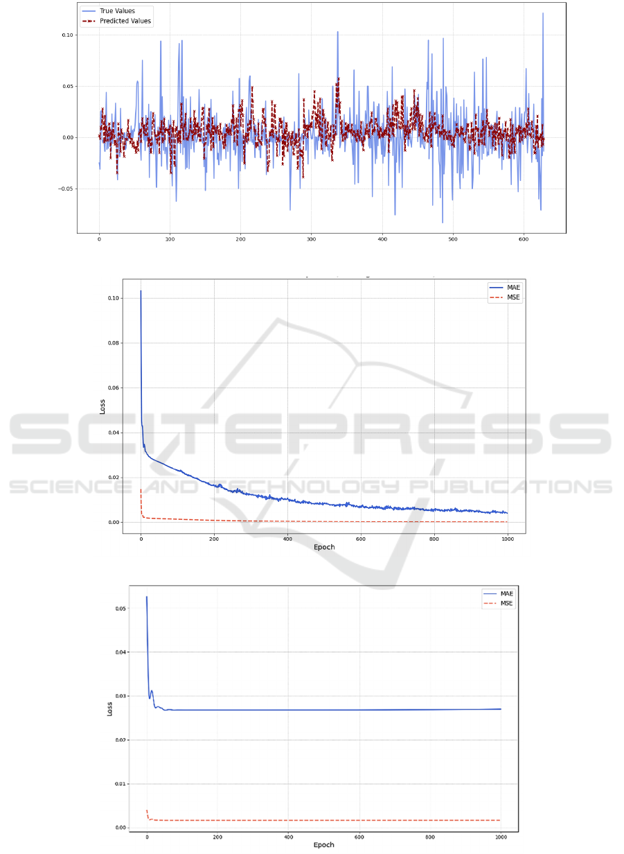
Figure 5: Predicted Returns from LSTM and Ground True (Photo/Picture credit: Original).

Figure 6: MAE & MSE of CNN over epochs (Photo/Picture credit: Original).

Figure 7: MAE & MSE of LSTM over epochs (Photo/Picture credit: Original).

Prediction of Daily Lognormal Returns for Bitcoin Based on LightGBM

161

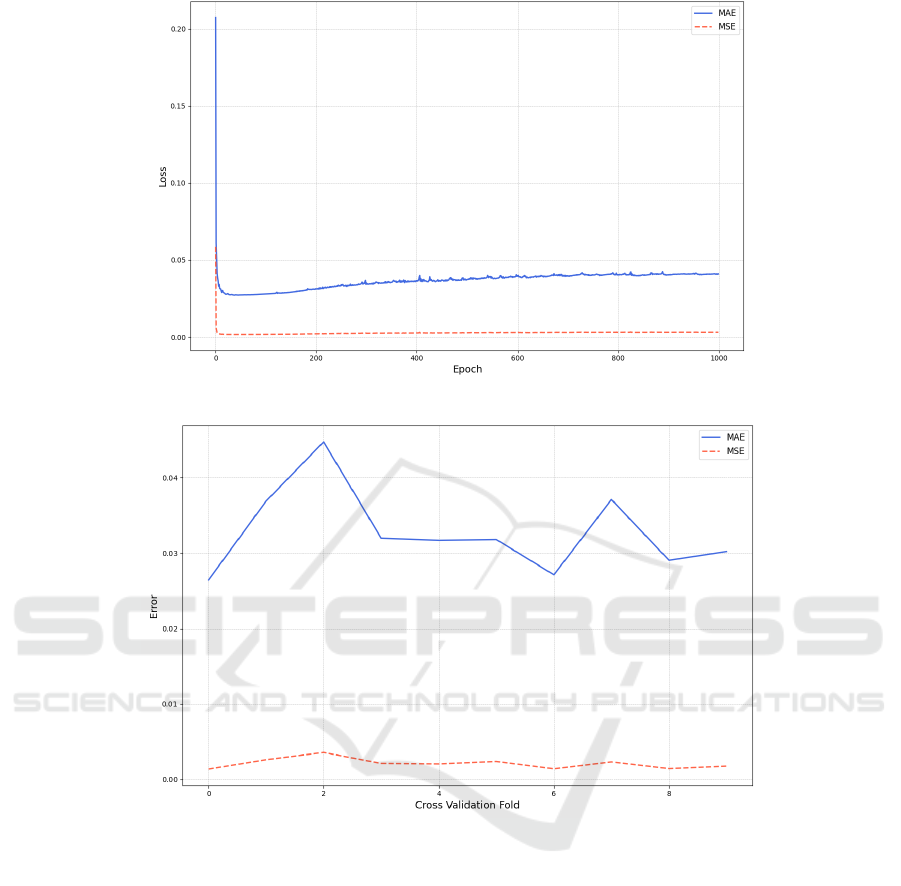
Figure 8: MAE & MSE of Transformer over epochs (Photo/Picture credit: Original).

Figure 9: MAE & MSE of LGBM over folds (Photo/Picture credit: Original).

3.4 Implications and Limitations

This research mainly focuses on evaluations of simple

pipelines. More sophisticate structures for these

pipelines are remained to be determined if they will

access better accuracy on the prediction task. The

relationship between the number of hidden layers and

output layers requires further confirmation. Aside of

that, different combination and connection between

components in algorithms may alternate the result,

which remains unverified during this research. The

embedding model proposed by the research consists

of the same structure as the basic Transformer and a

L2 regularization. On top of this pipeline, choosing

the output of one model as the input of another model

is an alternative method for embedding.

Theoretically, even the proposed model can better

fit the actual distribution of Bitcoin’s returns, the

explanatory of independent variables becomes a new

problem. Since each layer will resample and project

the original data into different dimensions, the

distribution of the input features shifts simultaneously.

The alternation hinders intuitive explanation on

features, which makes the framework hard to attribute

gain and loss to specific components.

4 CONCLUSIONS

The volatile risk of the Bitcoin introduces uncertainty

to investors that wish to hold Bitcoin for a mid-term

or long-term period. The daily return of the asset, as

ECAI 2024 - International Conference on E-commerce and Artiﬁcial Intelligence

162

this research has showcased, could potentially cause

unrealized loss to investors. Therefore, it is

reasonable for investors to utilize predictive model to

forecast huge volatility in an incoming short-term.

Researching results shows that neural network

models are capable to boost the performance in

prediction task by dynamically handling the financial

data both in a long-run period and an instantaneous

window. Yet there are plenty of space and

possibilities to increase R-squared by adding more

technique indicators that reveal the relationship

between historical prices and volumes, or by

implementing more elaborate calibration to existing

model to reduce noises in time-series data. Standing

on the ground of non-linearity, NN-based model such

as Transformer is worth highly attention from

investors that holding and trading Bitcoin less

frequently. It could be a possible choice for this type

of investor to lower their exposure to the volatile risk

by dynamically and seasonally training the NN-based

model for quick shifting market conditions and

utilizing it to foresee the deep risk in future returns.

REFERENCES

Alabdullah, A. A., Iqbal, M., Zahid, M., Khan, K., Amin,

M. N., Jalal, F. E., 2022. Prediction of rapid chloride

penetration resistance of metakaolin based high

strength concrete using light GBM and XGBoost

models by incorporating SHAP analysis. Construction

and Building Materials, 345, 128296.

Auer, R., Monnet, C., Shin, H. S., 2021. Permissioned

Distributed Ledgers and the Governance of Money. BIS

working papers, 21.

Beikverdi A, Song J., 2015. Trend of centralization in

Bitcoin’s distributed network. Software Engineering,

Artificial Intelligence, Networking and

Parallel/Distributed Computing SNPD, 2015 16th

IEEE/ACIS International Conference on p. 1–6.

D’Aliessi, Michele 2016, June 1. How does the blockchain

work? Retrieved from https://medium.com/@michel

edaliessi/how-does-the-blockchain-work98c8cd01d2ae

Dinh, T. T. A., Liu, R., Zhang, M., Chen, G., Ooi, B. C.,

Wang, J., 2018. Untangling blockchain: A data

processing view of blockchain systems. IEEE

Transactions on Knowledge and Data Engineering, 307,

1366–1385.

Farrell, M., 2013. Bitcoin prices surge post-Cyprus bailout.

Retrieved from:

http://money.cnn.com/2013/03/28/investing/bitcoin-

cyprus/index.html 53 Ferguson, N. 2009. The ascent of

money: A financial history of the world. New York:

Penguin Books.

Gorkhali, A., Shrestha, A., 2020. Blockchain: a literature

review. Journal of Management Analytics, 7(3), 321–

343.

Huang, X., Zhang, W., Tang, X., Zhang, M., Surbiryala, J.,

Iosifidis, V., Liu, Z., Zhang, J., 2021. LSTM Based

Sentiment Analysis for Cryptocurrency Prediction. In

Database Systems for Advanced Applications: 26th

International Conference, DASFAA 2021, Taipei,

Taiwan, April 11–14, 2021, Proceedings, Part III 26,

617-621.

Jiang, Z., Liang, J., 2017. Cryptocurrency portfolio

management with deep reinforcement learning. 2017

Intelligent systems conference (IntelliSys), 905-913.

Kang, K. Y., 2022. Cryptocurrency and double spending

history: transactions with zero confirmation. Economic

Theory, 752, 453–491.

Kar, S. K., 2023. A Deep Learning CNN based Approach to

the Problem of Crypto-Currency Prediction. Soft

Computing Research Society eBooks, 1123–1136.

Khattak, B. H. A., Shafi, I., Rashid, C. H., Safran, M.,

Alfarhood, S., Ashraf, I., 2024. Profitability trend

prediction in crypto financial markets using Fibonacci

technical indicator and hybrid CNN model. Journal of

Big Data, 111.

Labbaf Khaniki, M. A., Manthouri, M., 2023. Enhancing

Price Prediction in Cryptocurrency Using Transformer

Neural Network and Technical Indicators. Faculty of

Electrical Engineering, K.N. Toosi University of

Technology, Tehran, Iran.

Lahmiri, S., Bekiros, S., 2019. Cryptocurrency forecasting

with deep learning chaotic neural networks. Chaos,

Solitons and Fractals. 118. 35-40.

Livieris, I. E., Kiriakidou, N., Stavroyiannis, S., Pintelas, P.,

2021. An Advanced CNN-LSTM Model for

Cryptocurrency Forecasting. IElectronics, 10, 287.

Madey, R. S., 2017. A study of the history of cryptocurrency

and associated risks and threats. Master's thesis, Utica

College.

Nasirtafreshi, I., 2022. Forecasting cryptocurrency prices

using Recurrent Neural Network and Long Short-term

Memory. Data Knowledge Engineering, 139, 102009.

Tanrikulu, H. M., Pabuccu, H., 2024. The Effect of Data

Types' on the Performance of Machine Learning

Algorithms for Financial Prediction. arXiv preprint

arXiv:2404.19324.

Uras, L. M., Marchesi, M., Tonelli, R., 2020 Forecasting

bitcoin closing price series using linear regression and

neural networks models. arXiv preprint

arXiv:2001.01127, 2020.

Yli-Huumo, J., Ko, D., Choi, S., Park, S., Smolander, K.,

2016. Where Is Current Research on Blockchain

Technology: A Systematic Review. PLoS ONE, 1110,

e0163477.

Zhao, Y., Khushi, M., 2021. Wavelet Denoised-ResNet

CNN and LightGBM Method to Predict Forex Rate of

Change. School of Computer Science, the University of

Sydney, NSW, Australia.

Prediction of Daily Lognormal Returns for Bitcoin Based on LightGBM

163