Positioning Method of Four-Wheel Drive Robots Based on

Multi-Sensor Fusion and Improved Adaptive Monte Carlo Algorithm

Zhang Yi

, Li Beijun

1,*

and Shi Zhiqiang

School of Advanced Manufacturing Engineering, Chongqing University of Posts and Telecommunications,

Chongqing, China

China Assistive Devices and Technology Center, Beijing, China

Keywords: Adaptive Monte Carlo, Stratified Low Variance Sampling, KLD Sampling, Path Planning.

Abstract: This paper proposes an improved method for the traditional Adaptive Monte Carlo Localization (AMCL)

algorithm, addressing issues such as long computation time and poor real-time updating ability. In the

sampling phase, this method improves the traditional AMCL algorithm by using a parallel approach of

stratified low variance sampling and KLD sampling. Additionally, the improved AMCL algorithm is

integrated into the ROS-based SLAM package to reduce robot positioning errors and improve map accuracy

in unknown environments during simultaneous localization and mapping. It is also integrated into the ROS-

based navigation package to enhance robot's localization accuracy in known environments and optimize both

global and local path planning functionality when loading pre-built maps.

1 INTRODUCTION

Mobile robots have been integrated into society, but

with the development of society, higher requirements

are being put forward for the various performance of

robots, and autonomous operation of robots is one of

them, and autonomous positioning is one of the basic

tasks of autonomous operation. The autonomous

localization of robots is based on the pose estimation

of the previous moment, utilizing environmental

information and sensor data, and optimizing the

algorithm to obtain the pose estimation of the current

moment to locate the mobile robot.

The AMCL (Adaptive Monte Carlo Localization)

localization algorithm is the adaptive Monte Carlo

localization algorithm. It is a classic algorithm in

robot positioning algorithms, widely used in robot

positioning, navigation, and path planning. However,

the traditional AMCL algorithm has high

computational complexity and large computational

load, which cannot meet the real-time requirements of

autonomous mobile robots, autonomous driving, and

other scenarios that require high real-time

performance and quick response. Therefore, this

article proposes an improved AMCL algorithm to

shorten the calculation time of the localization

algorithm.

The main research content of this article is as

follows: In the sampling stage, the AMCL

localization algorithm has been improved, which

involves parallel implementation of Stratified Low

Variance Sampling and KLD sampling. The

improved AMCL localization algorithm not only

shortens the calculation time of localization, but also

improves the accuracy and real-time performance of

localization. At the same time, the improved AMCL

algorithm is loaded into the mapping and navigation

function package of the ROS system (Robot

Operating System). By adjusting the AMCL

parameters and resampling rules, higher precision

grid maps are created in unknown environments. At

the same time, global and local planning are used to

track the localization of robot humans.

2 FUSION LOCALIZATION

BASED ON IMPROVED AMCL

2.1 AMCL Algorithm

The AMCL algorithm is an improved version based

on the MCL (Monte Carlo Localization) algorithm,

which introduces an adaptive mechanism to improve

the accuracy and robustness of localization.

Beijun, L., Yi, Z. and Zhiqiang, S.

Positioning Method of Four-Wheel Drive Robots Based on Multi-Sensor Fusion and Improved Adaptive Monte Carlo Algorithm.

DOI: 10.5220/0012875700004536

Paper published under CC license (CC BY-NC-ND 4.0)

In Proceedings of the 1st International Conference on Data Mining, E-Learning, and Information Systems (DMEIS 2024), pages 10-16

ISBN: 978-989-758-715-3

Assuming the robot's pose is

, The observed

value is

1:t

z , input is

1:t

u , According to Bayesian

theorem, it can be obtained that:

1: 1: 1 1:

1: 1 1: 1 1:

(| , |,

|,)*

)( ,)

(( | ,*( )

tt ttt t

tt t

ttt

pxzu zxz u

xz u pzz u

−

−−

(1)

Among them,

()

1: 1:

ttt

px z u

is the pose state,

1: 1 1:

(,)|,

tt t t

pz x z u

−

is a sensor observation model,

111::

|(,)

tt t

−

is the motion model,

1: 1 1:

(| , )

tt t

zz u

−

is a normalized constant.

By using Bayesian filters, the above equation can

be expressed in recursive form:

() ( ) ( )

()

|* |,

ttttttt

bel x p z x p x u bel x dx

−−



(2)

Among them,

()

pz x

is the probability

density function, and

()

tt t

px ubelx

−

is the

motion model.

For particle filtering, use a set of state

assumptions

[] []

{

}

to approximate the

posterior distribution

()

1: 1:

ttt

px z u

, where

[]

the state assumption of the i-th particle,

[]

is the

weight of the i-th particle. By randomly sampling a

group of particles in the state space, a rough state

estimation can be obtained.

Predicting each particle based on the motion

model as the robot moves:

[] []

()

[]

|, ε

iii

ttttt

xpxxu

−

(3)

Among them,

[

]

is a random disturbance from

motion model noise.

When the robot receives sensor observations, the

weight of each particle is updated based on the sensor

model:

[] []

()

[]

()

|* |

ii i

ttt tt

pz x pz x

−









(4)

Among them,

[]

()

pz x

represents the

observation probability of the given particle position

by the sensor.

The particles and their corresponding weights are

resampled to update the state estimates. This process

can be done by randomly sampling from the current

particle distribution and generating a new set of

particles according to the particle weight distribution.

2.2 Stratified Low Variance Sampling

In the AMCL algorithm, the resampling process has

a significant impact on the accuracy and speed of the

algorithm, but traditional polynomial resampling

methods can lead to high variance in certain

situations, making the estimation results unstable; At

the same time, because polynomial resampling is

done through polynomial distribution, it can cause

some important samples to be discarded during the

resampling process, thereby affecting the accuracy of

the estimation. In order to ensure the stability and

accuracy of the algorithm, the stratified low variance

sampling method is selected in this paper.

The main idea of stratified low variance sampling

is to divide the population sample into several layers,

and then conduct random sampling in each layer, so

that the sample proportion of each layer is the same

as the population. This can ensure the

representativeness of the sample and reduce the

variance of the sample. Assuming we have N

particles, each with a weight of

w . We need to

resample these particles to obtain new N particles that

satisfy the relationship between weight and

probability density function. Firstly, normalize the

weights of all particles to obtain the probability

density function

ii j

pw w

−









(5)

Then integrate the probability density function

and calculate the cumulative distribution function:



(6)

Next, generate a random number

[0, )uN

−

∈

the starting point for the first sampled particle, and

define two variables j, k, both of which have an initial

value of 1.

Generate a uniformly distributed random number

()

rU N

−



and use the following formula for

resampling:

1, 1

if u r C

then x x

and j j k k

else x x







=+ =+





(7)

Repeat the above resampling until k>N.

Finally, set the weights of all new particles to

−

. This completes the entire hierarchical low variance

resampling process.

2.3 KLD Sampling

KLD sampling is a key technique for particle filter

adaptation and is commonly used to determine

Positioning Method of Four-Wheel Drive Robots Based on Multi-Sensor Fusion and Improved Adaptive Monte Carlo Algorithm

whether resampling is necessary. Its principle is

based on Kullback-Leibler divergence, which

measures the degree of difference between two

probability distributions and can be used to evaluate

the representativeness of particle sets. Assuming

there is a target particle collection for KLD sampling

to determine whether to resample, the weight of the

target particle is first calculated by normalizing the

particle weight:

()

qwsunw

−

(8)

Among them,

q represents the target weight of

particle i,

w represents the weight of particle i, and

()

un w

represents the sum of all particle weights.

Calculate the KL divergence between the

approximate distribution and the true distribution to

determine if they are close:

( ) () () ()

()

(

)

|| log *

LP Q Px Px Qx dx

−



(9)

Among them,

()

represents the probability

density of the true distribution at x, and

()

represents the probability density of the approximate

distribution at x.

Calculate the probability density function of an

approximate distribution, expressed as:

() ( )

()

Qx q x x

=−



(10)

Among them,

()

−

is the Dirac Delta

function, represented

x− , the value is 1, otherwise

it is 0.

Substitute the probability density function of the

approximate distribution into the KL divergence

formula and perform an integral operation on the

entire space:

()() () ()

()

(

)

|| log * *

LP Q Px Px q x x d

−



=−







(11)

Since the approximate distribution is represented

by a set of particles, we can introduce an importance

weight w_i for each particle. So that the approximate

distribution can be represented as:

() ( )

()

Qx w x x

=−



(12)

Substitute the probability density function of the

approximate distribution with importance weights

into the KL divergence formula and perform

integration operations on the entire space:

( ) () () ( )

()

(

)

|| log * *

LP Q Px Px w x x d

−



=−







(13)

Due to the properties of the Dirac Delta function,

the KL divergence formula can be further

transformed into:

( ) () ()

()

|| log * *

ieff

LP Q Px Px w x x

−



=−







(14)

Among them,

()()

()

eff i i i

xwxw

−



the weighted average position.

Define the number of effective particles

eff

is:

()

eff i

−



, and then based on the relationship

between KL divergence and the number of effective

particles, it can be determined whether resampling is

necessary.

2.4 AMCL Based on Parallel

Resampling and KLD Sampling

Traditional KLD sampling involves resampling at a

specific time and generating a new particle set after

resampling is completed. Then perform KLD

sampling on all particles one by one. When the

number of sampled particles reaches the required

number of particles according to the KLD criterion,

the remaining particles will not participate in

subsequent probability statistical operations, and the

KLD sampling of these particles will also be

terminated. Sampling termination requires

resampling and KLD sampling, which will greatly

increase calculation time and also cause positioning

delay. In order to shorten calculation time, improve

positioning accuracy and real-time performance, it is

proposed to parallelize resampling and KLD

sampling. In this method, a resampling operation is

first performed while calculating the KL divergence

of the particle set. Then, based on the results of KL

divergence, determine whether resampling is

necessary again.

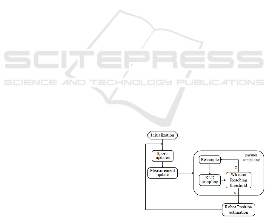
The AMCL algorithm process based on parallel

resampling and KLD sampling is as follows:

Figure 1: Improved AMCL Algorithm Process.

DMEIS 2024 - The International Conference on Data Mining, E-Learning, and Information Systems

1) Firstly, initialize the filter, collect and generate

an initial particle set, and assign equal weights to each

particle.

2) Based on the motion model of the robot, each

particle is sampled and predicted to update its state.

Assuming the linear velocity of the robot is v and the

angular velocity of the robot is ω, Sports updates are

as follows:

()

**cos

tt t

xxtv

=+Δ

(15)

()

**sin

tt t

yytv

=+Δ

(16)

θθ ω

=+Δ

(17)

Among them,

and

represents the position

coordinate of the robot at time t,

represents the

orientation angle of the robot at time t, and ∆t

represents the time step.

3) Update the weight of each particle based on the

sensor measurement information of the robot. Based

on the particle's location and map, use the

measurement model to calculate the probability

density function

()

pz x

of the particle under the

current measurement, and calculate the weight

w of

each particle by the total weight of all particles to

obtain the normalized weight

, and use the

normalized weight

as the final weight of

Based on the normalized weight of each particle

, resampling is performed to obtain a new particle

set

{

}

'' '

,,,

xx

. Then, the KLD calculation

method is used to compare the weight distribution of

the new particle set with the target weight

distribution, and the KLD value is calculated:

()

*log *

iii

KLD w w w

−







(18)

Among them,

represents the number of

particles obtained after resampling.

Then evaluate whether resampling is necessary

based on the set threshold. If the KLD value exceeds

the threshold, resampling is performed; On the

contrary, skip the resampling step.

5) Repeat steps 2 to 4 for motion updates,

measurement updates, parallel resampling, and KLD

calculations to gradually adjust the particle set.

6) Calculate the mean and variance of the robot's

position estimation:

hii



(19)

()

var *

hiih

wxx

=−



(20)

Among them,

represents the mean of robot

position estimation, and the

()

var

table represents

the variance of node position estimation.

The algorithm resampling and KL divergence

calculation are carried out in parallel, which can

determine whether resampling is necessary in a more

timely manner and reduce positioning delay.

Meanwhile, since the calculation of KL divergence is

performed before resampling, it is possible to

determine whether resampling is necessary before

resampling, avoiding unnecessary calculation time.

2.5 Improved AMCL Algorithm and

Multi-Sensor Fusion

Improved AMCL algorithm and multi-sensor fusion

steps:

Figure 2: Steps for Improving AMCL Algorithm and Multi

Sensor Fusion.

1) Data collection: Use an encoder to measure the

motion of robot wheels, in order to obtain the motion

model of the robot, including translation and rotation

information. At the same time, using LiDAR to

perceive the surrounding environment and obtain

environmental maps and obstacle information;

2) Motion prediction: Using encoder data to

predict the current position based on the robot's

motion model; Use LiDAR data for map matching

and particle filtering to obtain initial estimates of the

robot's position;

3) Perception update: Run steps 1 to 5 of the

resampling and KLD parallel AMCL algorithm every

time new LiDAR and encoder data is received to

obtain the estimated mean and variance of the

resampling particle set and robot position;

4) Data fusion: Using an extended Kalman filter,

the estimated values obtained from motion prediction

are combined with the measurement data of LiDAR

and encoder to obtain the final robot position

estimation result;

5) Output robot position estimation: Combining

the fused data, output the final robot position

estimation result, including the robot's position

Positioning Method of Four-Wheel Drive Robots Based on Multi-Sensor Fusion and Improved Adaptive Monte Carlo Algorithm

coordinates and corresponding uncertainty

information.

By utilizing the motion information of encoders

and the environmental perception of LiDAR through

multi-sensor fusion, the positioning accuracy and

robustness of robots have been greatly improved,

enabling them to calibrate and locate in complex

environments.

3 EXPERIMENTATION

3.1 Experimental Platform

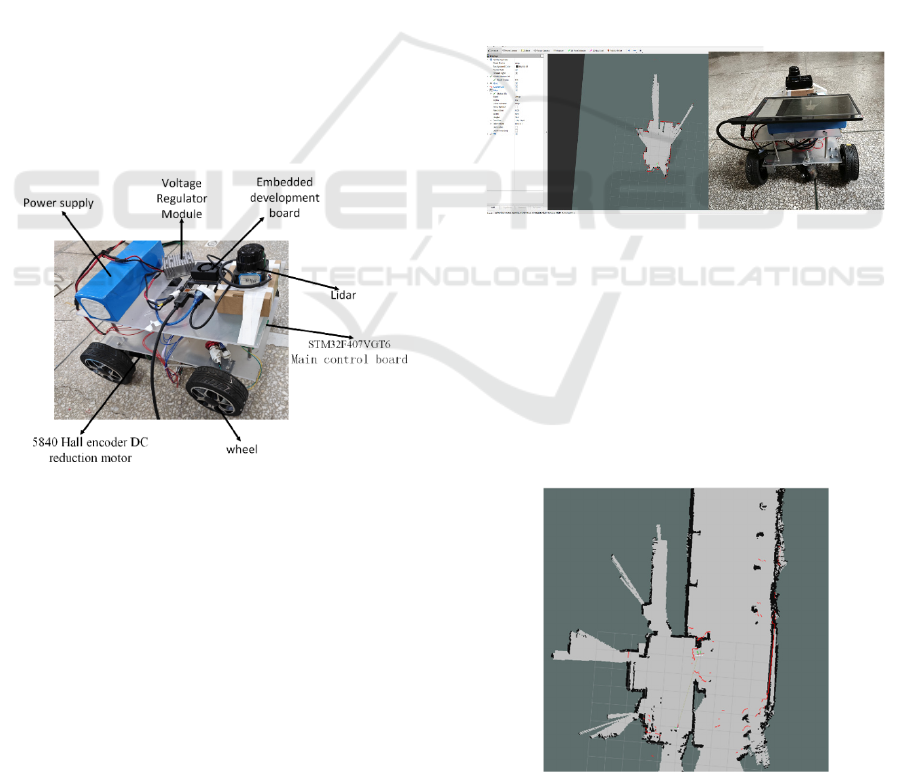
The mobile robot selected for this experiment is

shown in Figure 3. The mobile robot is equipped with

a 5840 Hall encoder DC deceleration motor that can

provide high speed, a Silan S1 LiDAR, and a 24V15A

lithium battery. The lower computer uses the

STM32F407VGT6 main control board to control the

low-level operation of the robot, while the upper

computer uses the NVIDIA high-performance

embedded development board. Install Ubuntu 20.04

environment and ROS open-source robot operating

system on the upper computer.

Figure 3: Overall Structure of the Robot.

3.2 Robot Localization Based on

AMCL Fusion Algorithm

This article selects the ROS system, which provides a

large number of functional packages that can be used

to handle common tasks of robots, such as sensor data

processing, navigation, motion control, perception,

etc. ROS adopts a distributed architecture, allowing

multiple independent software modules (referred to

as nodes) to communicate through information

transmission. This distributed communication, where

each node is independent of each other, greatly

improves the system's fault tolerance and

maintainability.

In the ROS environment, build an environment

map using the open-source SLAM algorithm

Gmapping feature pack. The selection of the mapping

environment is relatively simple, and the road surface

is relatively flat on the external corridor of the

laboratory. Firstly, test whether the entire system is

running normally. After everything is normal, start

the low-level control program of the robot, open the

communication node and Gmapping mapping node,

and simultaneously start the rviz node for

environmental visualization and keyboard control

program. Control the robot's movement through a

remote keyboard to scan environmental information.

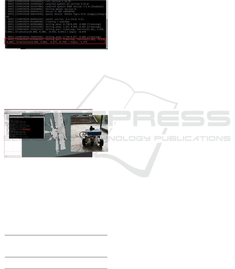
On the visualization interface of rviz, information

features of the surrounding environment can be seen.

After the robot completes a circle in the relevant

environment, it can complete map construction, as

shown in Figure 4.

Figure 4: SLAM Mapping Process.

After the map construction is completed, start the

map_ The server node saves the constructed map as a

two-dimensional grid map. The constructed two-

dimensional grid map is shown in Figure 5. During

the mapping process, the node continuously corrects

the robot's posture in the environment based on the

position estimation provided by the AMCL algorithm

and the information conveyed by sensors to ensure

the accuracy of map construction.

Figure 5: Built Grid Map.

DMEIS 2024 - The International Conference on Data Mining, E-Learning, and Information Systems

After the map construction is completed, start the

underlying communication nodes, navigation nodes,

and rviz visualization interface to assist in keyboard

control. After determining the initial position of the

robot, start setting navigation points on the map. The

process of setting navigation points is shown in

Figure 6.

Figure 6: Navigation Point Settings.

After completing the navigation point setting,

start the path planning node, and the robot will use

sensors such as LiDAR to start autonomous

navigation based on the node information. After

successful navigation, the window will prompt that

the node has been successfully reached, as shown in

Figure 7.

Figure 7: Robot Autonomous Navigation.

By comparing the error generated by using the

traditional AMCL algorithm for positioning, as

shown in Table 1, under the same environmental and

hardware conditions, using the traditional AMCL

algorithm for positioning resulted in a standard

deviation of 7.7cm, while using the algorithm

proposed in this paper resulted in a standard deviation

of 5.8cm.

Table 1: Positioning error statistics.

Positioning Method

Maximum

distance error

(cm)

Distance

standard

deviation

(

)

AMCL 32.4 7.7

Proposed Method 14.7 5.8

4 CONCLUSIONS

In this paper, the mathematical models of AMCL

algorithm, stratified low variance sampling and KLD

sampling are analyzed. Based on the goal of reducing

algorithm computation time and improving algorithm

real-time performance, it is determined to adopt the

AMCL algorithm with parallel hierarchical low

variance resampling and KLD sampling. This

algorithm improves the positioning accuracy of the

ROS system during SLAM mapping, and when

applied to the autonomous navigation module, it

assists in positioning and also improves the efficiency

of path planning. Of course, most of the sensors used

in this article are two-dimensional sensors. If you

want to achieve three-dimensional positioning, you

need to add three-dimensional sensors such as

cameras and three-dimensional LiDAR to perform

positioning in a three-dimensional environment.

ACKNOWLEDGEMENTS

1) Research Project of China Disabled Persons'

Federation – on Assistive Technology:

2022CDPFAT-01.

2) Chongqing Urban Management Research

Project (Chengguan Kezi 2022 No. 34).

REFERENCES

Wang, N., Wang, J., Li, L., J., 2019. An improved AMCL

robot positioning method. Journal of Navigation and

Positioning, vol.07, no.03, pp. 31- 37, Tongfang

HowNet (Beijing) Technology Co., Ltd,

https://doi.org/10.16547/j.cnki.10- 1096.20190306.

Chen, M., Zhang, S., Miao, C. and Li, Y., J., 2023. Self-

recovery Monte Carlo localization algorithm.

Optoelectronics · Laser, vol.34, no.01, pp.43-51,

Tongfang HowNet (Beijing) Technology Co., Ltd,

https://doi.org/10.16136/j.joel.2023.01.0169.

Li, Y. and Wu, M., J., 2023. An improved localization

method for indoor robots based on ultrasound and

AMCL. Agricultural Equipment and Vehicle

Engineering, vol.61, no.06, pp.117-121146, Tongfang

HowNet (Beijing) Technology Co., Ltd,

https://doi.org/10.39696/j.issn.1673-3142.2023.06.024

Zhang, S., Li, Y., Zhang, T., J., 2022. AMCL localization

algorithm based on fast affine template matching.

Journal of Beijing University of Aeronautics and

Astronautics, vol.221, no.04, pp.1-10, Tongfang

HowNet (Beijing) Technology Co., Ltd, https://

doi.org/10.13700/j.bh.1001-5965.2022.0001.

Jiang, L., Nie, W., Zhu, J., Liu, Q., Tian, T., Li, J., J., 2022.

Improved AMCL Relocation Algorithm Based on

Positioning Method of Four-Wheel Drive Robots Based on Multi-Sensor Fusion and Improved Adaptive Monte Carlo Algorithm

Semantic Maps with Corner Information. Journal of

Mechanical Engineering, vol.58, no.24, pp.312-323,

Tongfang HowNet (Beijing) Technology Co., Ltd,

https://doi.org/10.3901/JME.2022.24.312.

Feng, J., Pei, D., Zou, Y., Zhang, B. and Ding, P., J., 2021.

An Improved AMCL Algorithm Based on Robot

Laser Localization. Progress in Laser and

Optoelectronics, vol.58, no.20, pp.1-9, Tongfang

HowNet (Beijing) Technology Co., Ltd,

https://doi.org/10.3788/LOP202158.28003.

Wang, Z., Yan, B., Dong, M., Wang, J. and Sun, P., J.,

2022. A Wall Climbing Robot Positioning Method

Based on LiDAR and Improved AMCL. Journal of

Instrumentation, vol.43, no.12, pp.220-227, Tongfang

HowNet (Beijing) Technology Co., Ltd, https://doi.org

/10.19650/j.cnki.cjsi.J2210261.

Yuan, Q., Tian, X., Shen, S., J., 2022. Mobile robot

localization based on multi-sensor fusion. Computer

System Applications, vol.31, no.03, pp.136-142,

Tongfang HowNet (Beijing) Technology Co., Ltd,

https://doi.org/10.15888/j.cnki.csa.008390.

Yang, J., Lin, R., Wang, Z., Sun, L., J., 2016. Research

and Design of Motion Control Systems for Wheeled

Mobile Robots. Modern Electronic Technology, vol.39,

no.02, pp.22-27, Tongfang HowNet (Beijing)

Technology Co., Ltd, https://doi.org/10.16652/

j.issn.1004373x.2016.02.007.

Ren, P. and Li, W., J., 2021. Mobile robot localization

based on improved visual mileage calculation method.

Automation and Instrumentation, vol.36, no.07, pp.32-

37,63, Tongfang HowNet (Beijing) Technology Co.,

Ltd, https://doi.org/10.19557/j.cnki.1001-

9944.2021.07.006.

Zhou, X., Wu, T., Li, B. and Sun, J., J., 2022. Research on

four-wheel drive mobile robots based on ROS and PX4

flight control. Modern Electronic Technology, vol.45,

no.20, pp.177-182, Tongfang HowNet (Beijing)

Technology Co., Ltd, https://doi.org/10.

16652/j.issn.1004373x.2022.20.035.

DMEIS 2024 - The International Conference on Data Mining, E-Learning, and Information Systems