An Interpretable Machine Learning Approach for Identifying

Occupational Stress in Healthcare Professionals

Milena Seibert Fernandes

, Roberto Rodrigues Filho

, Iwens Sene-Junior

, Stefan Sarkadi

Alison R. Panisson

and Anal

ucia Schiafﬁno Morales

Department of Computing, Federal University of Santa Catarina, Santa Catarina, Brazil

Institute of Informatics, Federal University of Goi

as, Goi

ania, Brazil

Department of Informatics, King’s College London, London, U.K.

Keywords:

Interpretable ML, Stress, AI for Healthcare.

Abstract:

In the last few years, several scientiﬁc studies have shown that occupational stress has a signiﬁcant impact

on workers, particularly those in the healthcare sector. This stress is caused by an imbalance between work

conditions, the worker’s ability to perform their tasks, and the social support they receive from colleagues and

management professionals. Researchers have explored occupational stress as part of a broader study on af-

fective systems in healthcare, investigating the use of biomarkers and machine learning approaches to identify

early conditions and avoid Burnout Syndrome. In this paper, a set of machine learning (ML) algorithms was

evaluated using statistical data on biomarkers from the AffectiveRoad database to determine whether the use

of explanations can help identify stress more objectively. This research integrates explainability and machine

learning to aid in the identiﬁcation of various levels of stress, which has not been previously evaluated for the

domain of occupational stress. The Random Forest is the best-performing model for this assignment, followed

by k-Nearest Neighbors and Neural Network. Later, explainers were applied to the Random Forest, highlight-

ing feature importance, partial dependencies between characteristics, and a summary of the impact of features

on outputs based on their values.

1 INTRODUCTION

Over the last few years, we have studied occupational

stress as part of a comprehensive study on affective

systems in healthcare to improve decision-making.

In seeking alternatives for identifying stress, studies

have been conducted on physiological parameters that

can assist in the non-invasive identiﬁcation of occupa-

tional stress (Morales et al., 2022b), (Morales et al.,

2022c). In the ﬁeld of affective systems, it is empha-

sized that recognizing emotions is a complicated task

that requires techniques capable of helping to identify

various aspects. These include the intensity levels of

emotions, the types of emotions, the factors that trig-

ger these emotions, and behavioral and social factors

that may affect the expression or suppression of emo-

tional issues (Picard, 2000).

Psychological professionals can identify occupa-

tional stress early through standardized responses to

questionnaires. A unique way to identify and diag-

nose stress conditions has been used for several years

with this technique. Despite the validity of these

methods, there is a concern about subjective bias as

they may generate distortions in the results (Greene

et al., 2016). With the advancement of sensor tech-

nology, several studies have been conducted to iden-

tify stress using physiological signals and machine

learning techniques (Morales et al., 2022b): heart

rate, brain activity, skin response, body temperature,

blood activity, respiratory response, and muscle ac-

tivity, i.e., biomarkers. There are potential parame-

ters to assist in identifying biomarkers; in fact, many

wrist-worn wearables have been tested in data col-

lection in recent years, and their results have been

promising (Morales et al., 2022a). The biomarker-

based approach, however, does not show much trust

because stress identiﬁcation involves psychological,

physiological, and emotional aspects. Stress repre-

sents a coordinated activation of multiple biological

systems following the introduction of a stressful stim-

ulus (stressors) that represents a disruption of home-

ostasis or a perceived disruption (Potts et al., 2019).

Many studies have examined the association between

this point and ML algorithms in the scientiﬁc litera-

Fernandes, M., Filho, R., Sene-Junior, I., Sarkadi, S., Panisson, A. and Morales, A.

An Interpretable Machine Learning Approach for Identifying Occupational Stress in Healthcare Professionals.

DOI: 10.5220/0012591300003636

Paper published under CC license (CC BY-NC-ND 4.0)

In Proceedings of the 16th International Conference on Agents and Artiﬁcial Intelligence (ICAART 2024) - Volume 1, pages 499-506

ISBN: 978-989-758-680-4; ISSN: 2184-433X

499

ture (Morales et al., 2022c). According to Inam et al.

(2021), the complexity and sophistication of systems

involving artiﬁcial intelligence (AI) have grown to the

point where humans are not always capable of under-

standing the reasoning behind the decisions made by

ML mechanisms. This fact can be attributed to large

datasets composed of a massive volume of informa-

tion used to train and test increasingly complex sys-

tems (Linardatos et al., 2021). Presently, the ability

to interpret and understand the mechanisms behind

AI is essential for the validation of ML systems in

healthcare area (Montavon et al., 2018). Addition-

ally, Guidotti et al. (2018) highlight the possibility

of ML components making incorrect decisions with-

out providing the opportunity to detect the learning

problem. Systems that apply AI for decision-making

can be classiﬁed into one of the following three cate-

gories:

• Opaque Systems that do not offer any insight into

their algorithmic mechanisms, concealing their

internal knowledge from the user (Doran et al.,

2017; Guidotti et al., 2018);

• Interpretable Systems, whose algorithmic mech-

anisms can be analyzed by their users (Doran

et al., 2017);

• Understandable Systems that emit symbols al-

lowing user-guided explanations on how a conclu-

sion is reached (Doran et al., 2017);

Explainable Artiﬁcial Intelligence (XAI) refers to

methods and techniques that produce understand-

able and accurate models, highlighting why a model

reaches a speciﬁc decision. Therefore, solutions ob-

tained by artiﬁcially intelligent systems can be com-

prehended by humans, providing more transparency

and interpretability to instill trust in the results pro-

duced by AI-based solutions (Inam et al., 2021). It

can be uncomfortable to rely on a decision made with-

out any explanation (Doran et al., 2017; Miller, 2019).

The fact that humans are not always capable of under-

standing the results of black-box algorithms increases

the necessity for interpretability, transparency, and ex-

plainability of outputs generated by artiﬁcial intelli-

gence systems. These factors are crucial for humans

to comprehend and trust AI-based systems (Inam

et al., 2021). The ability of XAI to identify stress

biomarkers from a dataset of stress biomarkers gath-

ered from a study group would be a valuable study in

this ﬁeld. In this way, biomarker-based systems can

be made more reliable and the dataset can be opti-

mized, thereby allowing for the identiﬁcation of indi-

vidual stressors to be enhanced.

In this paper we present an evaluation of a set

of machine learning algorithms trained with statisti-

cal data of biomarkers available in the AffectiveRoad

database (Lopez-Martinez et al., 2019; Vos et al.,

2022) for the detection of different levels of stress.

In this study, we investigate whether explanations are

useful for identifying stress objectively. Biomarkers

used from the database are similar to those used to

identify occupational stress in healthworkers (Hos-

seini et al., 2022): heart rate (HR), electrodermal ac-

tivity (EDA), and skin temperature (TEMP). The ma-

chine learning algorithms used were Support Vector

Machine (SVM), k-Nearest Neighbors (kNN), Neu-

ral Network (NN), Random Forest (RF), and Logistic

Regression (LR). After identifying the algorithm with

the best performance, we presented explanations that

highlighted the characteristics of the dataset that have

the most inﬂuence on identifying stress. Explainers

employed for identiﬁcation were Partial Dependency

Plot, Feature Importance, and Summary Plot. Lastly,

model optimization was conducted considering only

the most important characteristics identiﬁed in the

previous stages. Finally, the algorithms and explain-

ers were tested and evaluated again for the optimized

dataset. The relevance of this research lies in com-

bining explainability and machine learning to assist

in the identiﬁcation of different levels of stress. Sim-

ilar works were identiﬁed in the scientiﬁc literature

(Chalabianloo et al., 2022; Tseng et al., 2020); how-

ever, no evidence was found of studies that evaluate

and explain machine learning methods speciﬁcally for

the domain of occupational stress. Thus, this present

study contributes to advancing knowledge in both the

ﬁeld of computer engineering (artiﬁcial intelligence)

and healthcare.

2 MATERIAL AND METHODS

From a preliminary study, articles from the scien-

tiﬁc literature were investigated to support the se-

lection criteria among publicly available databases

for occupational stress detection. Consideration was

given to the article by (Hosseini et al., 2022), which

utilizes the AffectiveRoad database (Lopez-Martinez

et al., 2019; Vos et al., 2022), and also provides pre-

processed data with 48 columns of statistical data on

the collected biomarkers.

For the selection of explainers, a study was con-

ducted in the scientiﬁc literature. Research such as

that by (Guidotti et al., 2018) and (Montavon et al.,

2018) present evidence for the use of explainers de-

pending on the model’s input and output. In the case

of this application for stress detection, good choices

to clearly highlight the reasons behind the model’s

decisions are explainers such as Summary Plot (SP),

EAA 2024 - Special Session on Emotions and Affective Agents

500

Partial Dependency Plot (PDP), and Feature Impor-

tance (FI). In addition, Shapley Additive Explana-

tors (Antwarg et al., 2021) were used to obtain such

explainers. Finally, the 10 most important character-

istics of the three models with the best performance

during the model evaluation stage were considered.

Therefore, all ﬁve algorithms were retrained three

times:

• First, with the 10 most important features for the

ﬁrst best result;

• Second, with the 10 most important features for

the second best result;

• Third, with the 10 most important features for the

third best result.

Therefore, three stages were developed: a prelim-

inary assessment of machine learning algorithms, an

explanation of the Random Forest algorithm, which

showed better performance during the evaluation, and

ﬁnally, training the algorithms with the most impor-

tant characteristics identiﬁed in the study. The dataset

has 49 columns.

3 RESULTS

A performance comparison of black-box machine

learning algorithms was conducted. A Python pro-

gram was developed to obtain statistics related to the

models’ performance, using classes from the sklearn

library to evaluate the selected algorithms in this

study. Furthermore, parameters indicating the per-

formance of each algorithm were obtained. These

parameters were Accuracy, AUC (area under ROC

curve), Recall, and F1 Score.

Figure 1 displays a diagram indicating the inputs

and potential outputs of the used algorithms.

Machine

Learning

Models

Heart rate data

Skin temperature

data

Electrodermal

activity data

Stress Levels

0 = no stress

1 = low stress

2 = high stress

k-Nearest Neighbors

Logistic Regression

Neural Network

Random Forest

Support Vector Machine

Figure 1: Diagram of inputs and outputs of the algorithms.

3.1 Evaluation of the Selected Machine

Learning Models

Among the biomarker data, totaling 48 input char-

acteristics, it includes the average of the last 11

measurement cycles, maximum value, minimum

value, and standard deviation of the three considered

biomarkers. Additionally, other data such as ampli-

tude, duration, kurtosis, standard deviation, and dis-

tortion of electrodermal activity, as well as the num-

ber of peaks and heartbeats per second of heart rate,

are included. On the other hand, the models’ output

is summarized by the stress level. There were three

levels of stress to classify and label: 0 (no stress), 1

(low stress), and 2 (a lot of stress).

3.1.1 Training of Models

The parameters used for training the algorithms were

also developed using the resources of the sklearn li-

brary. In the case of the Random Forest, some pa-

rameters were modiﬁed to follow the same settings

chosen by (Hosseini et al., 2022). In other cases, the

parameters were varied and chosen based on the al-

gorithms’ performance with parameter settings. The

following are the training parameters applied to each

model:

• k-Nearest Neighbors was trained with k being 5,

using Euclidean metric, and uniform weight.

• Logistic Regression was trained with L2 regular-

ization and C equal to 1.

• Neural Network was trained with 100 neurons in

hidden layers, ReLu activation, and Adam opti-

mization.

• Random Forest was trained with 100 trees and a

minimum number of branches set to 5.

• Support Vector Machine was trained with a cost

of 1, regression loss of 0.1, linear kernel, and nu-

merical tolerance of 0.001.

It’s worth noting that Support Vector Machine and

Logistic Regression algorithms are more commonly

used as binary classiﬁers, in applications with only

two possible outputs. For this reason, approaches

were employed to enable the models trained with

these algorithms to consider three classes. For the

Support Vector Machine algorithm, a One Vs. One

approach was used, where 3 classiﬁer models were

trained, each using data from two distinct classes.

Additionally, the Logistic Regression model used the

One Vs. Rest approach, so that three classiﬁers were

trained, with each considering one of the three possi-

ble outputs as positive and the other two as negative.

An Interpretable Machine Learning Approach for Identifying Occupational Stress in Healthcare Professionals

501

3.1.2 Results of Algorithm Evaluation

The algorithms were then tested, where 70% of the

data was selected for training in all cases, and the re-

maining 30% was used for testing. The division of

data for training and testing was randomly performed

using the train test split function from the sklearn li-

brary. The evaluation was conducted by comparing

the expected outputs with the outputs obtained by

each model.

Table 1 shows the results obtained after evaluating

the algorithms with the test data.

Table 1: Results of model evaluation.

Model AUC Accuracy F1 Recall

(1) RF 0.994 0.955 0.943 0.933

(2) kNN 0.964 0.878 0.854 0.854

(3) NN 0.900 0.771 0.702 0.691

(4) LR 0.747 0.610 0.453 0.496

(5) SVM 0.735 0.617 0.451 0.500

For all the parameters used, a value closer to 1 in-

dicates better performance. For this reason, the mod-

els were ranked in order of AUC, as observed in the

assigned ranking. This parameter was chosen because

it represents the relationship between true positives

and false positives classiﬁed by the models. Note that

the algorithms Logistic Regression and Support Vec-

tor Machine would change their ranking if the deci-

sive parameter were accuracy or recall.

Based on the AUC value, the Random Forest al-

gorithm presents excellent performance in classifying

stress levels using biomarkers. Also showing good

performance are the k-Nearest Neighbors and Neu-

ral Network algorithm. On the other hand, the Sup-

port Vector Machine and Logistic Regression algo-

rithms exhibit performance closer to a random clas-

siﬁer, making them less suitable for real-world appli-

cations.

3.2 Explanation of the Random Forest

As the Random Forest showed the best result, explain-

ers were applied to the trained model to elucidate how

the Random Forest works. The explainers were ob-

tained using the shap library.

3.2.1 The Shap Library

The shap library employs measures known as shap

values, introduced by (Lundberg and Lee, 2017).

These measures constitute a uniﬁed representation of

feature importance, based on Shapley Values, which

utilize game theory equations to derive values. While

Shapley Values quantify the contribution each player

brings to a game, shap values quantify the contri-

bution each feature brings to the model’s prediction,

making shap the most advanced explainability library

to date (Mazzanti, 2020).

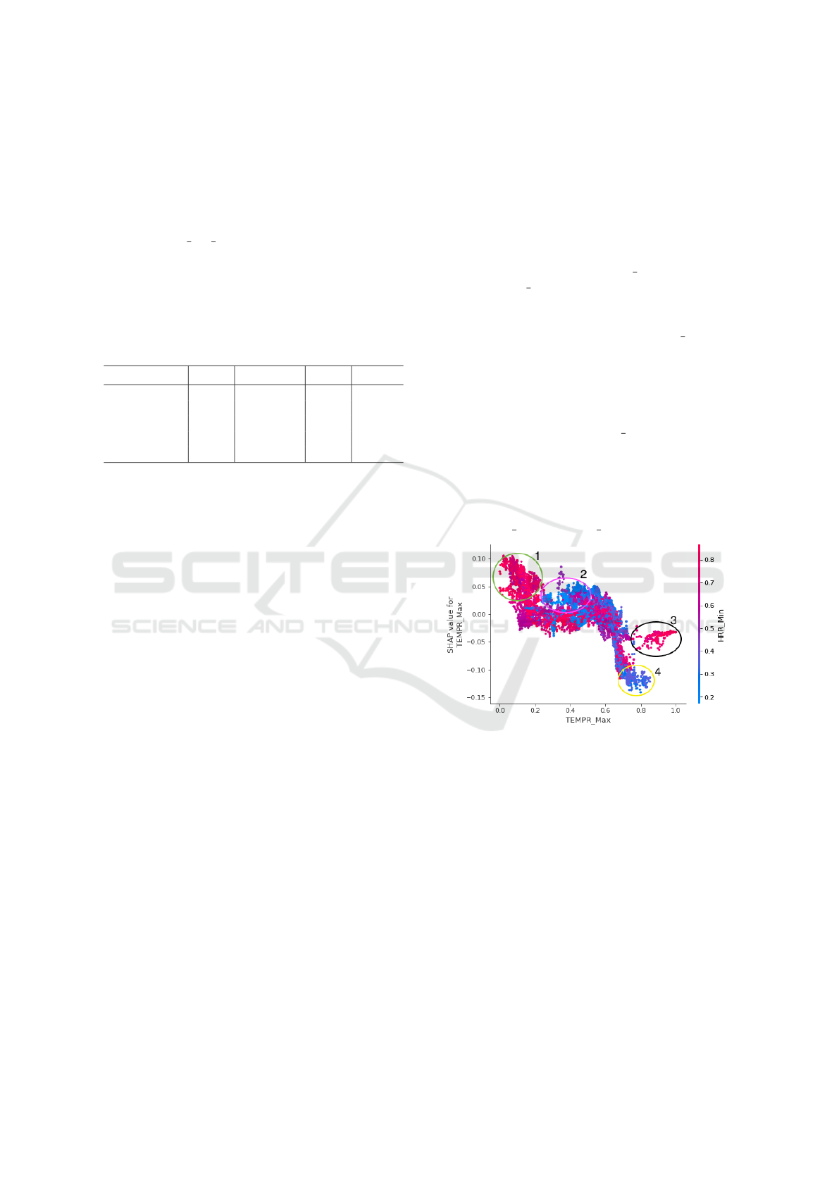
3.2.2 Partial Dependence Plot

Figure 2 depicts a partial dependence plot of the Ran-

dom Forest for the feature TEMPR Max, considering

the feature HRR Min when the considered output is 2

(high stress).

The horizontal axis of the graph represents the

proportion of values of the feature TEMPR Max, the

maximum value of skin temperature. The closer to

0.0, the closer it is to the smallest measured value for

this feature, and the closer to 1.0, the closer it is to the

largest measured value for this feature.

Similarly, the colors of the markers indicate the

proportion of the value of HRR Min, the minimum

value of heart rate. The more blue, the closer it is to

the minimum value measured for this feature, and the

closer to red, the closer it is to the maximum value

measured for this feature. Thus, the vertical axis indi-

cates the impact of the relationship between the fea-

tures TEMPR Max and HRR Min on the model.

Figure 2: Partial Dependence Plot of the model.

To increase understanding, four regions of the plot

deserving attention have been highlighted. These re-

gions are:

• Region 1 indicates that when the minimum heart

rate has a high value and the maximum skin tem-

perature has a low value, the skin temperature

feature positively contributes to detecting a stress

level of 2 (high stress).

• Region 2 suggests that as the minimum heart rate

decreases and the maximum skin temperature in-

creases, the impact of maximum skin temperature

decreases, approaching 0.

• Region 3 signiﬁes that high values of minimum

heart rate and maximum skin temperature have a

EAA 2024 - Special Session on Emotions and Affective Agents

502

small negative impact, contributing to diagnosing

little or no stress.

• Region 4 suggests that high values of maximum

skin temperature, combined with low values of

minimum heart rate, contribute to an output in-

dicative of little or no stress.

It is noteworthy that the partial dependence plot is

a type of local explanation, as it considers only one

target output.

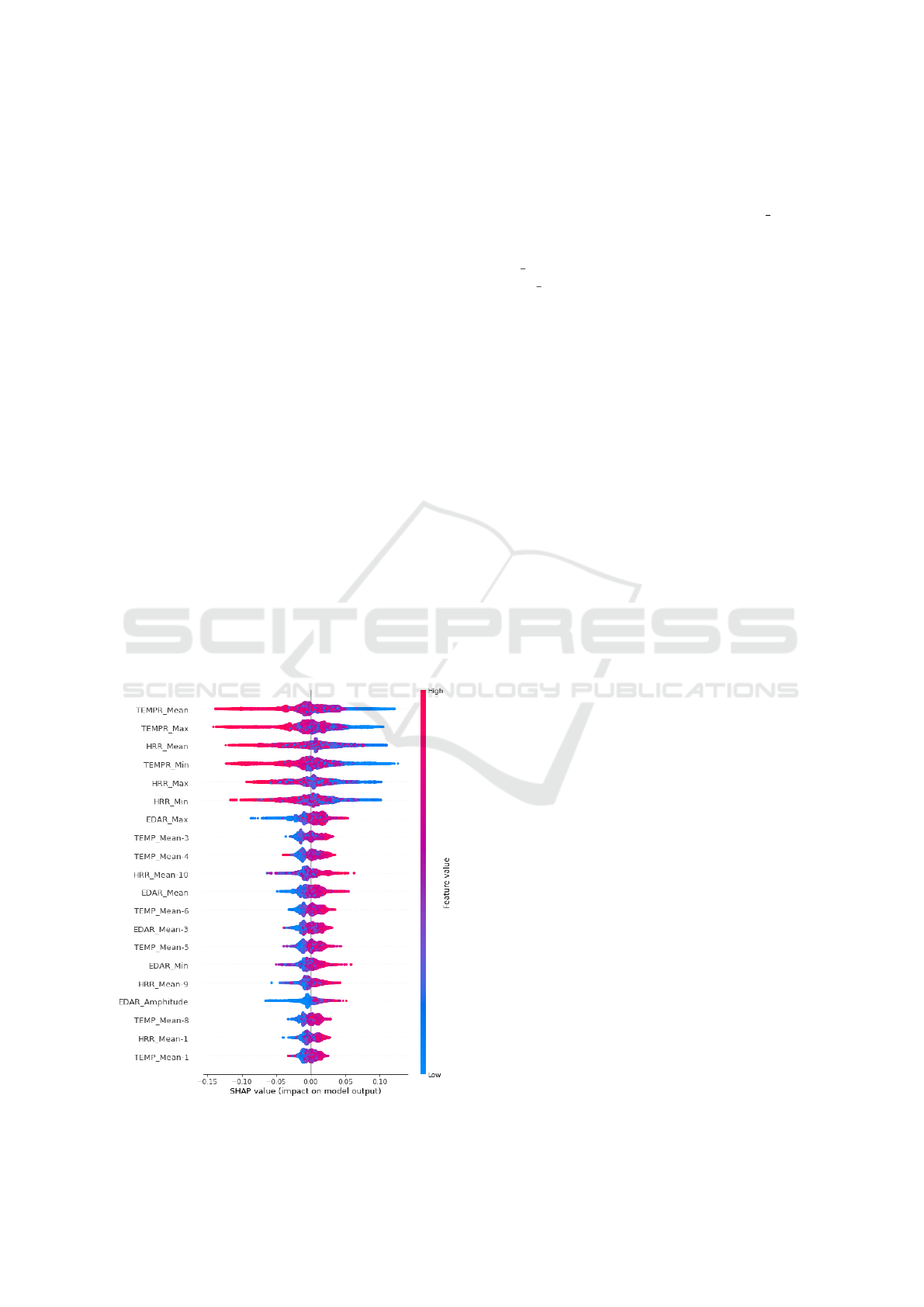
3.2.3 Summary Plot

The summary plot is named as such because it aims

to “summarize” the impact of features associated with

their values. Red points indicate that the feature value

is higher than most other values assigned to that fea-

ture. Similarly, blue points correspond to values lower

than most other values assigned to a particular feature.

Each row corresponds to a feature, indicated on the

left, and each point corresponds to a data instance.

The horizontal axis indicates the impact, positive

or negative, that the feature has on the considered out-

put value. In the middle of the plot, there’s a vertical

line indicating an impact of 0, where features do not

inﬂuence the model’s output. Points on the left have

a negative impact, while points towards the right have

a positive impact on the output considered. Figure 3

presents the summary plot of the Random Forest, con-

sidering output 2 (high stress).

Figure 3: Summary Plot of the Random Forest.

The plot highlights that the top six features are

crucial for the model’s output, as they possess more

than double the importance of the others. Addi-

tionally, it’s noticeable that the feature TEMP Mean,

i.e., average skin temperature, has the most signif-

icant impact on the result. Following closely are

TEMP Max, which is the maximum skin temperature,

and HRR Mean, representing the mean heart rate.

It can be noted that all the top six most important

features exhibit the same behavior: with low values,

the features contribute to the high stress output, while

with high values, there is a tendency towards diag-

noses of little or no stress.

It is also notable that concerning less important

features, the points are closer to the no-impact line,

and the relationship between the feature values and

their impact on the model’s output is unclear. More-

over, the summary plot is a local explanation, consid-

ering only one of the possible outputs. Next, the re-

sults of training the ﬁve models using only the top ten

most important features from the three models with

the best performance are presented.

3.3 Training Algorithms with Most

Important Features

As the ﬁnal stage of this work’s development, the

training of algorithms is conducted using the top 10

most important features for the three highest-rated

outcomes. Training with fewer features can help im-

prove model training time and evaluate which fea-

tures are truly necessary for occupational stress detec-

tion, enabling the simpliﬁcation of data preprocess-

ing. This investigation aims to verify if is it possible

to achieve similar results with fewer features in each

of the studied algorithms.

For training, it was necessary to ﬁrst ﬁnd the 10

most important features from the 3 best-performing

algorithms tested in the study: Random Forest, k-

Nearest Neighbors, and Neural Network. Figure 3

displays the feature importance assessment for the

Random Forest. The top 10 most relevant features for

k-Nearest Neighbors and Neural network were also

considered for training all ﬁve models. With this in-

formation, it was possible to perform the training of

the ﬁve algorithms again, using only the top ten fea-

tures from each Feature Importance analysis.

All ﬁve models were retrained, and the same per-

formance parameters were obtained. Table 2 shows

the AUC obtained from all the models trained with

sets of features.

The ﬁrst column of Table 2 displays the AUC

found for the models trained with all the features in

the dataset.

An Interpretable Machine Learning Approach for Identifying Occupational Stress in Healthcare Professionals

503

Table 2: AUC results from training with all features, and

the top 10 impactful features for Random Forest, k-Nearest

Neighbors and Neural Network.

Model All 10 RF 10 kNN 10 NN

(1) RF 0.994 0.992 0.986 0.991

(2) kNN 0.964 0.990 0.960 0.988

(3) NN 0.900 0.870 0.841 0.875

(4) LR 0.747 0.736 0.729 0.739

(5) SVM 0.735 0.735 0.720 0.732

The second column, 10 RF, displays the AUC

found for the models trained only with the 10 most

important features for Random Forest. When com-

paring the AUC value of models when trained with

the top 10 most important features of RF model with

the AUC of models trained with all features, it is ob-

served that there was no drastic reduction in the per-

formance of any of the models. On the other hand,

it is worth highlighting the signiﬁcant improvement

in the kNN model’s performance, which considerably

approaches the RF model, ranked ﬁrst. Additionally,

the classiﬁcation of the algorithms remains the same.

The third column, 10 kNN, displays the AUC

found for the models trained only with the 10 most

important features for k-Nearest Neighbors. When

comparing the results from training with the top

10 most important features of kNN model with the

results from training with all features, all models

showed a decrease in performance, but this decrease

was scarcely noticeable in practice.

Finally, the last column, 10 NN, displays the AUC

found for the models trained only with the 10 most

important features for Neural Network. These re-

sults show a slight deterioration in the performance

of all results compared to the performance of models

trained with all features, except for the kNN model.

Similar to what was observed in the results from train-

ing with the most impactful features for Random For-

est, the k-Nearest Neighbors model showed a signif-

icant improvement in performance, also approaching

the Random Forest in the top position. These results

also do not alter the classiﬁcation of the algorithms.

4 DISCUSSION

In this section, we present the main outcomes of this

study and compare and discuss them in relation to

ﬁndings from other works identiﬁed in the literature.

The primary outcome of the machine learning

algorithm evaluation stage was the superior perfor-

mance observed in the Random Forest model. In re-

lated studies (Dave et al., 2020), the XGBoost, a tree

ensemble model similar to Random Forest introduced

by (Chen and Guestrin, 2016), was included in evalu-

ations, unlike in this research.

Moreover, the research by (Tseng et al., 2020)

provided an assessment of machine learning algo-

rithms, concluding that the combination of XGBoost

with Random Forest into a single algorithm outper-

formed all other evaluated models, which included

SVM, LR, and simple decision trees. Additionally,

in (Tseng et al., 2020), XGBoost and Random For-

est ranked second and third, respectively, indicating

the strong performance of tree ensemble algorithms.

This research did not combine algorithms and did not

test XGBoost.

Additionally, in (Chalabianloo et al., 2022), four

classiﬁers were identiﬁed as the most promising for

training. These classiﬁers were SVM, Random For-

est, Extremely Randomized Tree, and Light Gradient

Boosting Machine, two of which are similar to those

used in this research. The latter two algorithms are

also tree-based ensemble methods, added to the study

after the authors observed promising results from the

Random Forest model. In this case, while Random

Forest was not chosen, it outperformed the others,

demonstrating its signiﬁcance.

Furthermore, the study by (Morales et al., 2022c)

provided a survey of machine learning model types,

considering the analyzed features for stress detection.

Despite SVM being a predominant model found in

many of the studies surveyed, it did not perform well

in this research with the utilized dataset and parame-

ters.

Conversely, in the work by (Bahani et al., 2021),

a comparison among machine learning models was

conducted, and the Random Forest exhibited one of

the worst performances among the evaluated algo-

rithms, which included SVM, kNN, NN, and Naive

Bayes. These results contrast with the outcomes of

the present study.

4.1 Comparing the Biomarker Impacts

This phase of the development resulted in an expla-

nation of the Random Forest, elucidating the signiﬁ-

cance of model characteristics, along with graphs as-

sociating their values and contributions to possible

outputs. Additionally, it ca be noted that the impor-

tance of characteristics varies depending on the algo-

rithm to be explained.

Among all the analyzed works, the only one ad-

dressing stress explainability, allowing for compar-

isons with the outcomes achieved in this study, is the

work by (Chalabianloo et al., 2022). On the other

hand, the work by (Hosseini et al., 2022) does not

provide explanations for the obtained outputs. Works

EAA 2024 - Special Session on Emotions and Affective Agents

504

such as (Madanu et al., 2022), (Pawar et al., 2020),

and (Dave et al., 2020) focus on different areas of

medicine, offering no possibility of comparing expla-

nations and biomarker impacts for occupational stress

detection.

The work by (Chalabianloo et al., 2022) uti-

lized data collected in a laboratory environment us-

ing seven different wearable devices. These data

were also categorized among low, medium, and high

stress through context analysis during their collec-

tion. Therefore, the quantity and types of data are

different from those used in this study. Feature se-

lection was performed using recursive feature elimi-

nation with cross-validation, resulting in 12 features

related to heart rate and entropy. The most important

features for the trained algorithms were the interval

between heartbeats and approximate entropy. Sub-

sequently, the authors added electrodermal activity

measures, resulting in improved model performance.

However, there is no presentation of the importance

of features associated with electrodermal activity, and

models trained with this data are not explained.

The work by (Chalabianloo et al., 2022) also in-

dicates that the importance of features varies accord-

ing to the explained model, which is supported by the

feature importance analysis conducted in this study.

Overall, it reinforces the signiﬁcance of features re-

lated to heart rate and electrodermal activity for stress

detection, emphasizing that the use of more biomark-

ers beyond heart rate contributes to making the model

more reliable.

4.2 Feature Reduction in Model

Training

Training with fewer features resulted in a slight re-

duction in the performance of the tested algorithms,

except for the k-Nearest Neighbors. When trained

with the 10 most important features from the Random

Forest and Neural Network algorithms, kNN showed

a signiﬁcant improvement in performance, showing

efﬁciency in cases with fewer features, as predicted

in the work by (Singh et al., 2016). Despite the per-

formance improvement, kNN did not outperform the

Random Forest in any case, which remained in the

ﬁrst position in all evaluations conducted. So far, no

research has been found in the survey that utilizes fea-

ture importance to reduce the dataset size and opti-

mize algorithm training.

Regarding training time, there was no noticeable

difference. However, it is noted that when training

algorithms with real-world data, much larger in size,

the difference may be noticeable. Training time tends

to be longer for LR and shorter for kNN, RF, and

SVM, or indifferent for NN according to character-

istics mentioned in the work by (Singh et al., 2016).

5 CONCLUSION

In this paper, we evaluate machine learning models

trained with statistical biomarker data extracted from

the AffectiveRoad database to detect different stress

levels. Our evaluation indicated Random Forest as

the best-performing model for this task, followed by

k-Nearest Neighbors and Neural Network. Later, ex-

plainers were applied to the Random Forest, high-

lighting partial dependencies between characteristics,

and a summary of the impact of features on outputs

based on their values.

The feature importance assessment suggests that

data related to skin temperature and heart rate hold

greater signiﬁcance for the model. Moreover, the

Random Forest summary graph indicates that high

values of skin temperature and heart rate suggest low

or no stress. Conversely, high electrodermal activity

indicates stress, although it holds less importance for

the model. Furthermore, the partial dependency graph

illustrates that even with high skin temperature, the

heart rate value can increase or decrease its impact on

the model. Noteworthy regions of the partial depen-

dency graph are highlighted to demonstrate how one

characteristic’s value inﬂuences the impact of another

characteristic.

Finally, this study presents some limitations.

Firstly, machine learning algorithm training was con-

ducted using only statistical features derived from

three biomarkers, while there are nine other biomark-

ers used in stress detection in other studies. Secondly,

some algorithms commonly used for diagnostics in

the healthcare ﬁeld were not part of the evaluation,

and no combination of algorithms was used for ﬁnal

assessment. Additionally, no emotional factor charac-

teristics were used for model training, making it difﬁ-

cult to distinguish between eustress and distress. Fur-

thermore, there was no translation of explanations to

make them easily understandable for healthcare pro-

fessionals, and there was no integration with a recom-

mendation system to address detected stress. Local

explanations, valid for only one data instance, can be

applied and translated into a sentence in natural lan-

guage to facilitate quicker and easier understanding of

these explanations.

An Interpretable Machine Learning Approach for Identifying Occupational Stress in Healthcare Professionals

505

REFERENCES

Antwarg, L., Miller, R. M., Shapira, B., and Rokach, L.

(2021). Explaining anomalies detected by autoen-

coders using Shapley Additive Explanations[Formula

presented]. Expert Systems with Applications, 186.

Bahani, K., Moujabbir, M., and Ramdani, M. (2021). An

accurate fuzzy rule-based classiﬁcation systems for

heart disease diagnosis. Scientiﬁc African, 14.

Chalabianloo, N., Can, Y. S., Umair, M., Sas, C., and Ersoy,

C. (2022). Application level performance evaluation

of wearable devices for stress classiﬁcation with ex-

plainable AI. Pervasive and Mobile Computing, 87.

Chen, T. and Guestrin, C. (2016). XGBoost: A scalable tree

boosting system. In Proceedings of the ACM SIGKDD

International Conference on Knowledge Discovery

and Data Mining, volume 13-17-August-2016, pages

785–794. Association for Computing Machinery.

Dave, D., Naik, H., Singhal, S., and Patel, P. (2020). Ex-

plainable AI meets Healthcare: A Study on Heart Dis-

ease Dataset. Technical report.

Doran, D., Schulz, S., and Besold, T. R. (2017). What Does

Explainable AI Really Mean? A New Conceptualiza-

tion of Perspectives.

Greene, S., Thapliyal, H., and Caban-Holt, A. (2016). A

survey of affective computing for stress detection:

Evaluating technologies in stress detection for bet-

ter health. IEEE Consumer Electronics Magazine,

5(4):44–56.

Guidotti, R., Monreale, A., Ruggieri, S., Turini, F., Gian-

notti, F., and Pedreschi, D. (2018). A survey of meth-

ods for explaining black box models. ACM Computing

Surveys, 51(5).

Hosseini, S., Gottumukkala, R., Katragadda, S., Bhupati-

raju, R. T., Ashkar, Z., Borst, C. W., and Cochran,

K. (2022). A multimodal sensor dataset for continu-

ous stress detection of nurses in a hospital. Scientiﬁc

Data, 9(1).

Inam, R., Terra, A., Mujumdar, A., Fersman, E., and Feljan,

A. V. (2021). Explainable AI – how humans can trust

AI.

Linardatos, P., Papastefanopoulos, V., and Kotsiantis, S.

(2021). Explainable ai: A review of machine learn-

ing interpretability methods.

Lopez-Martinez, D., El-Haouij, N., and Picard, R. (2019).

Detection of Real-world Driving-induced Affective

State Using Physiological Signals and Multi-view

Multi-task Machine Learning.

Lundberg, S. and Lee, S.-I. (2017). A Uniﬁed Approach to

Interpreting Model Predictions.

Madanu, R., Abbod, M. F., Hsiao, F.-J., Chen, W.-T., and

Shieh, J.-S. (2022). Explainable AI (XAI) Applied

in Machine Learning for Pain Modeling: A Review.

Technologies, 10(3):74.

Mazzanti, S. (2020). SHAP Values Explained Exactly How

You Wished Someone Explained to You.

Miller, T. (2019). Explanation in artiﬁcial intelligence: In-

sights from the social sciences.

Montavon, G., Samek, W., and M

uller, K. R. (2018). Meth-

ods for interpreting and understanding deep neural

networks.

Morales, A., Barbosa, M., Mor

as, L., Cazella, S. C., Sgobbi,

L. F., Sene, I., and Marques, G. (2022a). Occupational

stress monitoring using biomarkers and smartwatches:

A systematic review. Sensors, 22(17).

Morales, A. S., de Oliveira Ourique, F., Mor

as, L. D.,

Barbosa, M. L. K., and Cazella, S. C. (2022b). A

Biomarker-Based Model to Assist the Identiﬁcation

of Stress in Health Workers Involved in Coping with

COVID-19, pages 485–500. Springer International

Publishing, Cham.

Morales, A. S., de Oliveira Ourique, F., Mor

as, L. D., and

Cazella, S. C. (2022c). Exploring Interpretable Ma-

chine Learning Methods and Biomarkers to Classify-

ing Occupational Stress of the Health Workers, pages

105–124. Springer International Publishing, Cham.

Pawar, U., O’shea, D., Rea, S., and O’reilly, R. (2020). Ex-

plainable AI in Healthcare. Technical report.

Picard, R. W. (2000). Affective computing. MIT press.

Potts, S. R., McCuddy, W. T., Jayan, D., and Porcelli, A. J.

(2019). To trust, or not to trust? individual differ-

ences in physiological reactivity predict trust under

acute stress. Psychoneuroendocrinology, 100:75–84.

Singh, A., Thakur, N., and Sharma, A. (2016). A Review of

Supervised Machine Learning Algorithms.

Tseng, P. Y., Chen, Y. T., Wang, C. H., Chiu, K. M., Peng,

Y. S., Hsu, S. P., Chen, K. L., Yang, C. Y., and Lee, O.

K. S. (2020). Prediction of the development of acute

kidney injury following cardiac surgery by machine

learning. Critical Care, 24(1).

Vos, G., Trinh, K., Sarnyai, Z., and Azghadi, M. R. (2022).

Machine Learning for Stress Monitoring from Wear-

able Devices: A Systematic Literature Review.

EAA 2024 - Special Session on Emotions and Affective Agents

506