Semantic Properties of Cosine Based Bias Scores for Word Embeddings
Sarah Schr
¨
oder
a
, Alexander Schulz
b
, Fabian Hinder
c
and Barbara Hammer
d
Machine Learning Group, Bielefeld University, Bielefeld, Germany
Keywords:
Language Models, Word Embeddings, Social Bias.
Abstract:
Plenty of works have brought social biases in language models to attention and proposed methods to detect
such biases. As a result, the literature contains a great deal of different bias tests and scores, each introduced
with the premise to uncover yet more biases that other scores fail to detect. What severely lacks in the literature,
however, are comparative studies that analyse such bias scores and help researchers to understand the benefits
or limitations of the existing methods. In this work, we aim to close this gap for cosine based bias scores.
By building on a geometric definition of bias, we propose requirements for bias scores to be considered
meaningful for quantifying biases. Furthermore, we formally analyze cosine based scores from the literature
with regard to these requirements. We underline these findings with experiments to show that the bias scores’
limitations have an impact in the application case.
1 INTRODUCTION
In the domain of Natural Language Processing (NLP),
many works have investigated social biases in terms
of associations in the embeddings space. Early works
(Bolukbasi et al., 2016; Caliskan et al., 2017) intro-
duced methods to measure and mitigate social biases
based on cosine similarity in word embeddigs. With
NLP research progressing to large language mod-
els and contextualized embeddings, doubts have been
raised whether these methods are still suitable for fair-
ness evaluation (May et al., 2019) and other works
criticize that for instance the Word Embedding As-
sociation Test (WEAT) (Caliskan et al., 2017) fails
to detect some kinds of biases (Gonen and Goldberg,
2019; Ethayarajh et al., 2019). Overall there exists a
great deal of bias measures in the literature, which not
necessarily detect the same biases (Kurita et al., 2019;
Gonen and Goldberg, 2019; Ethayarajh et al., 2019).
In general, researchers are questioning the usability of
model intrinsic bias measures, such as cosine based
methods (Steed et al., 2022; Goldfarb-Tarrant et al.,
2020; Kaneko et al., 2022). There exist few papers
that compare the performance of different bias scores
(Delobelle et al., 2021; Schr
¨
oder et al., 2023) and
works that evaluate experimental setups for bias mea-
a
https://orcid.org/0000-0002-7954-3133
b
https://orcid.org/0000-0002-0739-612X
c
https://orcid.org/0000-0002-1199-4085
d
https://orcid.org/0000-0002-0935-5591
surement (Seshadri et al., 2022). However, to our
knowledge, only two works investigate the properties
of intrinsic bias scores on a theoretical level (Etha-
yarajh et al., 2019; Du et al., 2021). To further close
this gap, we evaluate the semantic properties of co-
sine based bias scores, focusing on bias quantification
as opposed to bias detection. We make the following
contributions: (i) We formalize the properties of trust-
worthiness and comparability as requirements for co-
sine based bias scores. (ii) We analyze WEAT and the
Direct Bias, two prominent examples from the liter-
ature. (iii) We conduct experiments to highlight the
behavior of WEAT and the Direct Bias in practice.
Both our theoretical analysis and experiments
show limitations of these bias scores in terms of bias
quantification. It is crucial that researchers take these
limitations into account when considering WEAT or
the Direct Bias for their works. Furthermore, we lay
the ground work to analyze other cosine based bias
scores and understand how they can be useful for the
fairness literature. The paper is structured as follows:
In Section 2 we summarize WEAT, the Direct Bias
and general terminology for cosine based bias mea-
sures from the literature. We introduce formal re-
quirements for such bias scores in Section 3 and ana-
lyze WEAT and the Direct Bias in terms of these re-
quirements in Section 4. In Section 5 we support our
theoretical findings by experiments, before drawing
our conclusions in Section 6.
160
Schröder, S., Schulz, A., Hinder, F. and Hammer, B.
Semantic Properties of Cosine Based Bias Scores for Word Embeddings.
DOI: 10.5220/0012577200003654
Paper published under CC license (CC BY-NC-ND 4.0)
In Proceedings of the 13th International Conference on Pattern Recognition Applications and Methods (ICPRAM 2024), pages 160-168
ISBN: 978-989-758-684-2; ISSN: 2184-4313
Proceedings Copyright © 2024 by SCITEPRESS – Science and Technology Publications, Lda.

2 RELATED WORK FOR BIAS IN
WORLD EMBEDDINGS
2.1 WEAT
The Word Embedding Association Test, short WEAT,
(Caliskan et al., 2017), is a statistical test for stereo-
types in word embeddings. The test compares two
sets of target words X and Y with two sets of bias at-
tributes A and B of equal size n under the hypothesis
that words in X are rather associated with words in A
and words in Y rather associated with words in B. The
association of a single word w with the bias attribute
sets A and B including n attributes each, is given by
s(w,A,B) =
1
n
∑
a∈A
cos(w,a) −
1
n
∑
b∈B
cos(w,b). (1)
To measure bias in the sets X and Y, the effect size is
used, which is a normalized measure for the associa-
tion difference between the target sets
d(X,Y,A,B) =
1
n
∑
x∈X
s(x,A,B) −
1
n
∑
y∈Y
s(y,A,B)
stddev
w∈X∪Y
s(w,A,B)
. (2)
A positive effect size confirms the hypothesis that
words in X are rather stereotypical for the attributes
in A and words in Y stereotypical for words in B,
while a negative effect size indicates that the stereo-
types would be counter-wise. To determine if the ef-
fect is indeed statistically significant, the permutation
test
p = P
r
[s(X
i
,Y
i
,A, B) > s(X ,Y,A,B)]. (3)
with subsets (X
i
,Y
i
) of X ∪Y and the test statistic
s(X,Y,A,B) =
∑
x∈X
s(x,A, B) −
∑
y∈Y
s(y,A, B)(4)
is done. As a statistical test WEAT is suited to confirm
a hypothesis (such that a certain type of stereotype
exists in a model), but it cannot prove the opposite.
2.2 Direct Bias
The Direct Bias (Bolukbasi et al., 2016) is defined as
the correlation of neutral words w ∈ W with a bias
direction (for example gender direction g):
DirectBias(W ) :=
1
|W |
∑
w∈W
|cos(w, g)|
c
(5)
with c determining the strictness of bias measure-
ment. The gender direction is either obtained by a
gender word-pair e.g. g = he −she or - to get a more
robust estimate - it is obtained by computing the first
principal component over a set of individual gender
directions from different word-pairs.
In terms of their debiasing algorithm the authors
describe how to obtain a bias subspace given defining
sets D
1
, ..., D
n
. A defining set D
i
includes words w
that only differ by the bias relevant topic e.g. for gen-
der bias {man,woman} could be used as a defining
set. Given these sets, the authors construct individ-
ual bias directions w − µ
i
∀w ∈ D
i
,i ∈ {1,...,n} and
µ
i
=
∑
w∈D
i
w
|D
i
|
. To obtain a k-dimensional bias sub-
space B they compute the k first principal components
over these samples.
2.3 Terminology
In the literature geometrical bias is measured by com-
paring neutral targets against sensitive attributes. By
targets and attributes we refer to vector representa-
tions of words, sentences or text in a d-dimensional
embedding space. However, the methodology can be
applied to any kind of vector representations. While
the exact notation varies between publications, we
summarize and use it in the following Sections as fol-
lows:
Given a protected attribute like gender or race, we
select n ≥ 2 protected groups that might be subject
to biases. Each protected group is defined by a set of
attributes a
ik
∈ A
i
with i ∈ {1,..., n} the group’s index.
We summarize these attribute sets as A = {A
1
,..., A
n
}.
The intuition is that the attributes define the relation of
protected groups by contrasting specifically over the
membership to the different groups. Therefore, it is
important that any attribute a
ik
∈ A
i
has a counterpart
a
jk
∈ A
j
∀ A
j
∈ A, j ̸= i that only differs from a
ik
by
the group membership. For instance, if we used A
1
=
{she, f emale,woman} as a selection of female terms,
A
2
= {he,male,man} would be the proper choice of
male terms.
Analogously to WEAT’s definition of word biases,
we define the association of a target t with one pro-
tected group, represented by A
i
, as
s(t,A
i
) =
1
|A
i
|
∑
a
ik
∈A
i
cos(t.a
ik
) (6)
A similar notion is found with the Direct Bias (Boluk-
basi et al., 2016). To detect bias, one would con-
sider the difference of associations towards the dif-
ferent groups, i.e. is t more similar to one protected
group than the others. This concept is also found in
most cosine based bias scores.
Whether such association differences are harmful de-
pends on whether t is theoretically neutral to the pro-
tected groups. For example, terms like ”aunt” or ”un-
cle” are associated with one or the other gender per
definition, while a term like ”nurse” should not be as-
sociated with gender.
Semantic Properties of Cosine Based Bias Scores for Word Embeddings
161

3 FORMAL REQUIREMENTS
FOR BIAS SCORES
3.1 Formal Bias Definition and
Notations
As baseline for our bias score requirements and the
following analysis of bias scores from the literature,
we suggest two intuitive definitions of individual bias
for target samples (e.g. one word) t and aggregated
biases for sets of targets T . For samples t we apply
the intuition of WEAT, extended to n protected groups
instead of only two.
Definition 3.1 (Individual Bias). Given n protected
groups represented by attribute sets A
1
, ..., A
n
and a
target t that is theoretically neutral to these groups,
we consider t biased if
∃A
i
,A
j
∈ A : s(t,A
i
) > s(t, A
j
) (7)
Definition 3.2 (Aggregated Bias). Given n protected
groups represented by attribute sets A
1
, ..., A
n
and a
set of targets T containing only samples that are theo-
retically neutral to these groups, we consider T biased
if at least one sample t ∈ T is biased:
∃A
i
,A
j
∈ A,t ∈ T : s(t,A
i
) > s(t, A
j
) (8)
The idea behind Definition 3.2 is that even when
looking at aggregated biases, each individual bias is
important, i.e. as long as there is one biased target in
the set, we cannot call the set unbiased, even if target
biases cancel out on average or the majority of targets
is unbiased.
In the following we will use a notation for bias
score functions in general: b(t,A) measuring the bias
of one target and b(T,A) for aggregated biases. Note
that there are two different strategies in the liter-
ature: Bias scores measuring bias over all neutral
words jointly (Direct Bias), which matches our nota-
tion b(T, A), and bias scores measuring the bias over
two groups of neutral words X,Y ⊂ T (WEAT). In
the later case, we consider the selection of subsets
X,Y ⊂ T as part of the bias score and thus treat it
as a function b(T,A).
Since the bias scores from the literature have dif-
ferent extreme values and different values indicating
no bias, we use the following notations: b
min
and b
max
are the extreme values of b(·) and b
0
is the value of
b(·) that means t or T is unbiased. Note that b
min
and
b
0
are not necessarily equal.
3.2 Requirements for Bias Metrics
Based on the definitions of bias explained in Sec-
tion 3.1, we formalize the properties of trustworthi-
ness and magnitude-comparability. The goal of both
properties is to ensure that biases can be quantified in
a way such that bias scores can be safely compared
between different embedding models and debiasing
methods can be evaluated without risking to overlook
bias.
3.2.1 Comparability
The goal of magnitude-comparability, is to ensure
that bias scores are comparable between embeddings
of different models. This is necessary to make state-
ments about embedding models being more or less bi-
ased than others, which includes comparing debiased
embeddings with their original counterparts. We find
a necessary condition for such comparability is the
possibility to reach the extreme values b
min
and b
max
of b(·) in different embedding spaces depending only
on the neutral targets and their relation to attribute
vectors, as opposed to the attribute vectors them-
selves, which might be embedded differently given
different models.
Definition 3.3 (Magnitude-Comparable). We call the
bias score function b(T,A) Magnitude-Comparable if,
for a fixed number of target samples in set T (includ-
ing the case T = {t}), the maximum bias score b
max
and the minimum bias score b
min
are independent of
the attribute sets in A:
max
T,|T |=const
b(T,A) = b
max
∀ A, (9)
min
T,|T |=const
b(T,A) = b
min
∀ A. (10)
3.2.2 Trustworthiness
The second property of trustworthiness defines
whether we can trust a bias score to report any bias
in accordance to Definitions 3.1 and 3.2, i.e. the
bias score can only reach b
0
, which indicates fairness,
if the observed target is equidistant to all protected
groups and for target sets if all samples in the ob-
served set of targets are unbiased. This is important,
because even if a set of targets is mostly unbiased or
target biases cancel out on average, individual biases
can still be harmful and should thus be detected. The
requirement for the consistency of the minimal bias
score b
0
can be formulated in a straight forward way
using the similarities to the attribute sets A
i
.
Definition 3.4 (Unbiased-Trustworthy). Let b
0
be the
bias score of a bias score function, that is equivalent
to no bias being measured. We call the bias score
function b(t,A) Unbiased-Trustworthy if
b(t,A) = b
0
⇐⇒ s(t,A
i
) = s(t, A
j
) ∀ A
i
,A
j
∈ A.
(11)
ICPRAM 2024 - 13th International Conference on Pattern Recognition Applications and Methods
162

Analogously for aggregated scores with a set T =
{t
1
,..., t
m
}, we say b(T,A) is Unbiased-Trustworthy
if
b(T,A) = b
0
(12)
⇐⇒ s(t
k
,A
i
) = s(t
k
,A
j
) ∀ A
i
,A
j
∈ A,k ∈ {1,..., m}.
(13)
4 ANALYSIS OF BIAS SCORES
As a major contribution of this work, we formally an-
alyze WEAT and the Direct Bias with regard to the
properties defined in Section 3.2. Table 1 gives an
overview over the properties. The detailed analyses
follow in Section 4.1 for WEAT and Section 4.2 for
the Direct Bias.
4.1 Analysis of WEAT
In the following, we detail properties of WEAT in
light of the definitions stated above. First, we focus
on the individual biases as reported by s(t,A,B).
Theorem 1. The bias score function s(t, A,B) of
WEAT is not Magnitude-Comparable.
Proof. With
ˆ
a =
1
|A|
∑
a∈A
a
||a||
and
ˆ
b analogously de-
fined, we can rewrite
s(t,A, B) =
t ·
ˆ
a
||t||
−
t ·
ˆ
b
||t||
(14)
=
t
||t||
·

ˆ
a −
ˆ
b

(15)
= cos(t,
ˆ
a −
ˆ
b)||
ˆ
a −
ˆ
b||. (16)
Hence we can show that the extreme values depend
on the attribute sets A and B:
max
t
s(t,A, B) = ||
ˆ
a −
ˆ
b||, (17)
min
t
s(t,A, B) = −||
ˆ
a −
ˆ
b|| (18)
The statement follows.
Theorem 2. The bias score function s(t, A,B) of
WEAT is Unbiased-Trustworthy.
Table 1: Overview over the properties of bias scores.
bias score comparable trustworthy
WEAT
sample
x ✓
WEAT ✓ x
DirectBias ✓ x
Proof. This follows directly from the definition of
s(t,A, B) (equation (1)):
s(t,A, B) = s(t, A) − s(t, B) = 0 (19)
⇐⇒ s(t,A) = s(t,B) (20)
Next, we focus on the properties of the effect size
d(X,Y, A,B), identified by WEAT in Table 1. Note
that it is not specified for cases, where s(t,A,B) =
s(t
′
,A, B) ∀t, t
′
∈ X ∪Y due to its denominator. This is
highly problematic considering Definition 3.4, which
states that a bias score should be 0 in that specific
case. For Theorem 4 we need Lemma 1 from the Ap-
pendix.
Theorem 3. The effect size d(X,Y,A, B) of WEAT is
not Unbiased-Trustworthy.
Proof. For the WEAT score b
0
= 0. With four
targets t
1
,t
2
,t
3
,t
4
and s(t
1
,A, B) = s(t
3
,A, B) and
s(t
2
,A, B) = s(t
4
,A, B) the effect size
d({t
1
,t
2
},{t
3
,t
4
},A, B) = (21)
(s(t
1
,A, B) + s(t
2
,A, B)) − (s(t
3
,A, B) + s(t
4
,A, B))
2 · stddev
t∈{t
1
,t
2
,t
3
,t
4
}
s(t,A, B)
(22)
is 0, if s(t
1
,A, B) ̸= s(t
2
,A, B) (otherwise d is not de-
fined). Now, for the simple case A = {a},B = {b}
and assuming all vectors having length 1, we see
s(t
1
,A, B) = s(t
3
,A, B)
⇐⇒ a · t
1
− b · t
1
= a · t
3
− b · t
3
⇐⇒ a · (t
1
− t
3
) − b ·(t
1
− t
3
) = 0
⇐⇒ (a − b)· (t
1
− t
3
) = 0. (23)
This implies that, if the two vectors a − b and t
1
− t
3
are orthogonal (and e.g. s(t
2
,A, B) = 0), the WEAT
score returns 0. In this case, there exist a,b, t
1
,t
3
with
s(t
1
,A, B) = s(t
3
,A, B) ̸= 0 and accordingly s(t
1
,A) ̸=
s(t
1
,B).
Theorem 4. The effect size d(X,Y,A,B) of
WEAT with X = {x
1
,. .. ,x
m
},Y = {y
1
,. .. ,y
m
}
is Magnitude-Comparable.
Proof. With c
i
= s(x
i
,A, B), c
i+m
= s(y
i
,A, B), n =
2m, ˆµ = 1/n
∑
n
i=1
c
i
and
ˆ
σ =
p
1/n
∑
n
i=1
(c
i
− µ)
2
, we
have
d =
1/m
∑
m
i=1
c
i
− 1/m
∑
2m
i=m+1
c
i
ˆ
σ
(24)
=
∑
m
i=1
c
i
−
∑
2m
i=m+1
c
i
+
∑
m
i=1
c
i
−
∑
m
i=1
c
i
m
ˆ
σ
=
2
∑
m
i=1
c
i
− 2mˆµ
m
ˆ
σ
=
2
m
m
∑
i=1
c
i
− ˆµ
ˆ
σ
∈ [−2,2] (25)
Semantic Properties of Cosine Based Bias Scores for Word Embeddings
163

where the last statement follows from Lemma 1 (see
Appendix) with
∑
m
i=1
c
i
−ˆµ
ˆ
σ
∈ [−m,m]. The extreme
value ±2 is reached if c
1
= ... = c
m
= −c
m+1
=
.. . = −c
2m
, which can be obtained by setting x
1
=
.. . = x
m
= −y
1
= . .. = −y
m
, independently of A
and B as long as A ̸= B and
∑
a
i
∈A
a
i
/∥a
i
∥ ̸= 0 ̸=
∑
b
i
∈B
b
i
/∥b
i
∥.
The proof of Theorem 4 shows that the effect size
reaches its extreme values only if all x ∈ X achieve
the same similarity score s(x,A, B) and s(y,A, B) =
−s(x,A, B) ∀ y ∈ Y , i.e. the smaller the variance
of s(x, A,B) and s(y,A,B) the higher the effect size.
This implies that we can influence the effect size by
changing the variance of s(t,A, B) without changing
whether the groups are separable in the embedding
space. Furthermore, the proof of Theorem 3 shows
that WEAT can report no bias even if the embeddings
contain associations with the bias attributes. This
problem occurs, because WEAT is only sensitive to
the stereotype ”X is associated with A and Y is asso-
ciated with B” and will overlook biases diverting from
this hypothesis.
4.2 Analysis of the Direct Bias
For the Direct Bias, the following theorems show
that it is Magnitude-Comparable, but not Unbiased-
Trustworthy. The proof for Theorem 6 shows that
the first principal component used by the Direct Bias
does not necessarily represent individual bias direc-
tions appropriately. This can lead to both over- and
underestimation of bias by the Direct Bias.
Theorem 5. The DirectBias is Magnitude-
Comparable for c ≥ 0.
Proof. For c ≥ 0 the individual bias |cos(t,g)|
c
is in
[0,1]. Calculating the mean over all targets in T does
not change this bound. The statement follows.
Theorem 6. The DirectBias is not Unbiased-
Trustworthy.
Proof. For the Direct Bias b
0
= 0 indicates no bias.
Consider a setup with two attribute sets A
=
{a
1
,a
2
}
and C = {c
1
,c
2
}.
Using the notation from Section 2.2 this gives us two
defining sets D
1
= {a
1
,c
1
} D
2
= {a
2
,c
2
}. Let a
1
=
(−x,rx)
T
= −c
1
,a
2
= (−x,−rx)
T
= −c
2
and r > 1.
The bias direction is obtained by computing the first
principal component over all (a
i
− µ
i
) and (c
i
− µ
i
)
with µ
i
=
a
i
+c
i
2
= 0. Due to r > 1, b = (0, 1)
T
is a
valid solution for the 1st principal component as it
maximizes the variance
b = argmax
∥v∥=1
∑
i
(v · a
i
)
2
+ (v · c
i
)
2
. (26)
According to the definition in Section 3.1, any
word t = (0,w
y
)
T
would be considered neutral to
groups A and C with s(t,A) = s(t,C) and being
equidistant to each word pair {a
i
,c
i
}.
But with the bias direction b = (0,1)
T
the Direct Bias
would report b
max
= 1 instead of b
0
= 0, which con-
tradicts Definition 3.4.
On the other hand, we would consider a word t =
(w
x
,0)
T
maximally biased, but the Direct Bias would
report no bias. Showing that the bias reported for sin-
gle words t is not Unbiased-Trustworthy, proves that
the DirectBias is not Unbiased-Trustworthy.
5 EXPERIMENTS
In the experiments, we show that the limitations of
WEAT and Direct Bias shown in Section 4 do oc-
cur with state-of-the-art language models. We show
that the effect size of WEAT can be misleading when
comparing bias in different settings. Furthermore,
we highlight how attribute embeddings differ between
different models, which impacts WEAT’s individ-
ual bias, and that the Direct Bias can obtain a mis-
leading bias direction by using the Principal Compo-
nent Analysis (PCA). We use different pretrained lan-
guage models from Huggingface (Wolf et al., 2019)
and the PCA implementation from Scikit-learn (Pe-
dregosa et al., 2011) and observe gender bias based
on 25 attributes per gender, such as (man,woman).
5.1 Weat’s Effect Size
In a first experiment, we demonstrate that the effect
size does not quantify social bias in terms of the sep-
arability of stereotypical targets. We use embeddings
of distilbert-base-uncased and openai-gpt to compute
gender bias according to s(t,A,B) and the effect size
d(X,Y, A,B) for stereotypically male/female job ti-
tles. Figure 1 shows the distribution of s(t,A,B) for
DistilBERT, where stereotypical male/female targets
are clearly distinct based on the sample bias. Figure
2 shows the distribution of s(t, A,B) for GPT, where
stereotypical male and female terms are similarly dis-
tributed. First, we focus on the DistilBERT model
(Figure 1), which clearly is biased with regard to the
tested words. We compare two cases with different
targets, such that the stereotypical target groups are
better separable in one case (left plot), which one may
describe as more severe or more obvious bias com-
pared to the second case, where the target groups are
almost separable (right plot). However, the effect size
behaves contrary to this.
Despite this, when comparing Figures 1 and 2 ,
ICPRAM 2024 - 13th International Conference on Pattern Recognition Applications and Methods
164

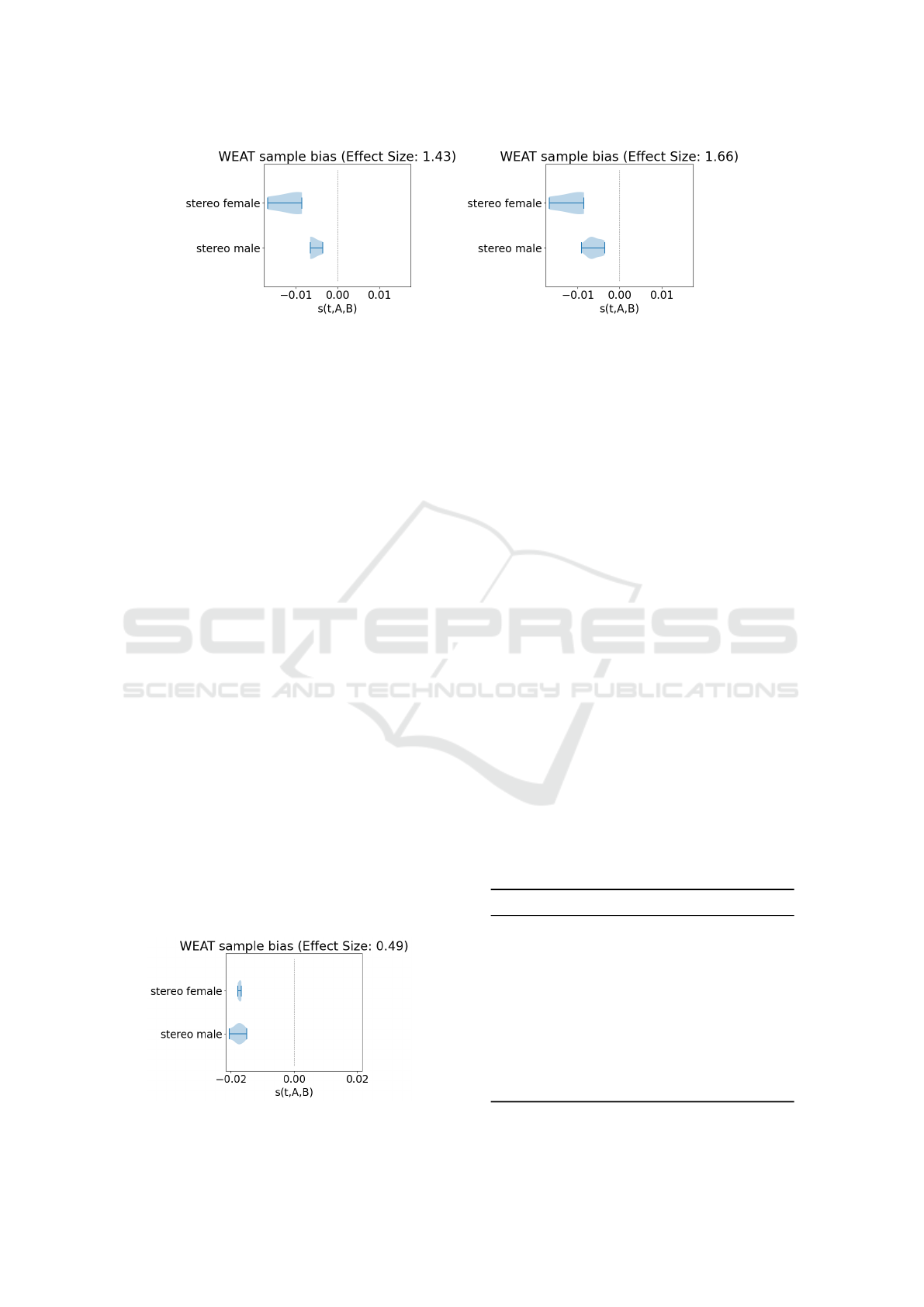
Figure 1: WEAT individual bias and effect size for distilBERT with different selections of target words. When selecting a
smaller number of job titles (left), we observe that stereotypical male/female jobs are more distinct w.r.t. s(t,A,B), while the
effect size is lower.
one can assume that large differences in effect sizes
still reveal significant differences in social bias. While
high effect sizes are reported in cases where both
stereotypical groups are (almost) separable, we report
low effect sizes when groups achieve similar individ-
ual biases. Furthermore, one should always report the
p-value jointly with the effect size to get an impres-
sion on its significance. In other terms, WEAT is use-
ful for qualitative bias analysis (or confirming biases),
but not quantitatively.
5.2 Weat’s Individual Bias
In Theorem 1 we discussed that WEAT’s individ-
ual bias depends on the mean difference of attributes
||
ˆ
a −
ˆ
b||. As shown in Table 2 these vary a lot be-
tween different language models. We report the two
most extreme values of 0.198 for distilroberta-base
and 5.206 for xlnet-base-uncased. With such dif-
ferences we cannot compare sample biases based on
their magnitude between different models.
5.3 Direct Bias
Figure 3 shows the correlation of different bias di-
rections on bert-base-uncased embeddings. We re-
port bias directions of individual word pairs such as
(man,woman) (left plot: 0-24, right plot: 0-22) and
the resulting bias direction as obtained by PCA (last
row). Overall we report very low correlations be-
Figure 2: WEAT’s individual bias for job titles in GPT.
tween the individual bias directions. The first prin-
cipal component reflects mostly individual bias direc-
tion 23 and 24 (left plot), which differ a lot from all
other bias directions. On contrary, if we excluded
word pairs 23 and 24 from the PCA (right plot), the
first principal component would give a better estimate
of bias directions 0-22. This shows that only one or
few ”outlier” pairs are sufficient to make the Direct
Bias measure ”bias” in a completely different way.
From a practical point of view, by analyzing the corre-
lation between individual bias directions we can get a
good estimate whether the first principal component is
a good estimate. Moreover, if we observe only weak
correlations between bias directions from the selected
word pairs, that is an indication that a 1-dimensional
bias direction may not be sufficient to capture the re-
lationship of sensitive groups with regard to which we
want to measure bias. While Bolukbasi et al. (Boluk-
basi et al., 2016) did not explicitly define that case for
the Direct Bias, they proposed to use a bias subspace,
defined by the k first principal components, for their
Debiasing algorithm, which is related to the Direct
Bias. Accordingly, this could be applied to the Direct
Bias. Apart from that, one should verify how well
the bias direction or bias subspace obtained by PCA
Table 2: Mean attribute difference ||
ˆ
a−
ˆ
b|| for different lan-
guage models given 25 attribute pairs for gender.
Model Name Mean Attribute Diff
openai-gpt 0.728
gpt2 0.842
bert-large-uncased 1.123
bert-base-uncased 0.568
distilbert-base-uncased 0.433
roberta-base 0.235
distilroberta-base 0.198
electra-base-generator 0.518
albert-base-v2 1.123
xlnet-base-cased 5.206
Semantic Properties of Cosine Based Bias Scores for Word Embeddings
165

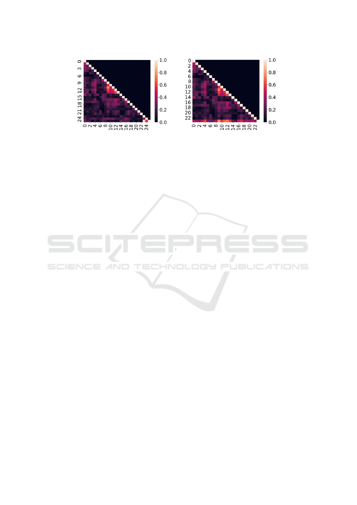
Figure 3: Correlation bias directions of individual word pairs (left: 0-24, right: 0-22) and the first principal component (last
row) as selected for the Direct Bias. The lowest row in the heatmap shows the correlation of individual bias directions with
the first principal component.
represents individual bias directions to make sure that
they’re actually measuring bias in the assumed way.
6 CONCLUSION
In this work, we introduce formal properties for co-
sine based bias scores, concerning their meaningful-
ness for quantification of social bias. We show that
WEAT and the Direct Bias have theoretical flaws that
limits their ability to quantify bias. Furthermore, we
show that these issues have a real impact when ap-
plying these bias scores on state-of-the-art language
models. These findings should be considered in the
experimental design when evaluating social bias with
one of these measures. Future works could build on
the proposed properties to analyze other scores from
the literature or propose a score that is better suited
for bias quantification. The findings of our theoretical
analysis open the question, whether the limitations of
cosine based scores reported in the literature are due
to the theoretical flaws of distinct scores, which are
highlighted by our analysis, rather than limitations of
geometrical properties as a sign of bias. This is an
important question that should be addressed in future
work. In general, we encourage other researchers to
take an effort to bring the various bias measures from
the literature into context and to highlight their prop-
erties and limitations, which is critical to derive best
practices for bias detection and quantification.
ACKNOWLEDGEMENTS
Funded by the Ministry of Culture and Science of
North-Rhine-Westphalia in the frame of the project
SAIL, NW21-059A.
REFERENCES
Bolukbasi, T., Chang, K.-W., Zou, J. Y., Saligrama, V., and
Kalai, A. T. (2016). Man is to computer programmer
as woman is to homemaker? debiasing word embed-
dings. Advances in neural information processing sys-
tems, 29:4349–4357.
Caliskan, A., Bryson, J. J., and Narayanan, A. (2017). Se-
mantics derived automatically from language corpora
contain human-like biases. Science, 356(6334):183–
186.
Delobelle, P., Tokpo, E. K., Calders, T., and Berendt, B.
(2021). Measuring fairness with biased rulers: A sur-
vey on quantifying biases in pretrained language mod-
els. arXiv preprint arXiv:2112.07447.
Du, Y., Fang, Q., and Nguyen, D. (2021). Assessing the
reliability of word embedding gender bias measures.
In Proceedings of the 2021 Conference on Empiri-
cal Methods in Natural Language Processing, pages
10012–10034, Online and Punta Cana, Dominican
Republic. Association for Computational Linguistics.
Ethayarajh, K., Duvenaud, D., and Hirst, G. (2019). Under-
standing undesirable word embedding associations.
arXiv preprint arXiv:1908.06361.
Goldfarb-Tarrant, S., Marchant, R., S
´
anchez, R. M.,
Pandya, M., and Lopez, A. (2020). Intrinsic bias
metrics do not correlate with application bias. arXiv
preprint arXiv:2012.15859.
Gonen, H. and Goldberg, Y. (2019). Lipstick on a pig: De-
biasing methods cover up systematic gender biases in
word embeddings but do not remove them. CoRR,
abs/1903.03862.
Kaneko, M., Bollegala, D., and Okazaki, N. (2022). De-
biasing isn’t enough!–on the effectiveness of debias-
ing mlms and their social biases in downstream tasks.
arXiv preprint arXiv:2210.02938.
Kurita, K., Vyas, N., Pareek, A., Black, A. W., and
Tsvetkov, Y. (2019). Measuring bias in con-
textualized word representations. arXiv preprint
arXiv:1906.07337.
May, C., Wang, A., Bordia, S., Bowman, S. R., and
Rudinger, R. (2019). On measuring social biases in
sentence encoders. CoRR, abs/1903.10561.
ICPRAM 2024 - 13th International Conference on Pattern Recognition Applications and Methods
166

Pedregosa, F., Varoquaux, G., Gramfort, A., Michel, V.,
Thirion, B., Grisel, O., Blondel, M., Prettenhofer,
P., Weiss, R., Dubourg, V., et al. (2011). Scikit-
learn: Machine learning in python. Journal of ma-
chine learning research, 12(Oct):2825–2830.
Schr
¨
oder, S., Schulz, A., Kenneweg, P., and Hammer, B.
(2023). So can we use intrinsic bias measures or not?
In Proceedings of the 12th International Conference
on Pattern Recognition Applications and Methods.
Seshadri, P., Pezeshkpour, P., and Singh, S. (2022). Quanti-
fying social biases using templates is unreliable. arXiv
preprint arXiv:2210.04337.
Steed, R., Panda, S., Kobren, A., and Wick, M. (2022). Up-
stream mitigation is not all you need: Testing the bias
transfer hypothesis in pre-trained language models. In
Proceedings of the 60th Annual Meeting of the Associ-
ation for Computational Linguistics (Volume 1: Long
Papers), pages 3524–3542.
Wolf, T., Debut, L., Sanh, V., Chaumond, J., Delangue, C.,
Moi, A., Cistac, P., Rault, T., Louf, R., Funtowicz,
M., and Brew, J. (2019). Huggingface’s transformers:
State-of-the-art natural language processing. CoRR,
abs/1910.03771.
APPENDIX
In order to show that the effect size of WEAT is
Magnitude-Comparable (see Theorem 4), we need
the following lemma.
Lemma 1. Let x
1
,..., x
n
∈ R be real numbers. Let
ˆµ,
ˆ
σ denote the empirical estimate of mean and stan-
dard deviation of the x
i
. Then, for any selection of
indices i
1
,..., i
m
, with i
j
̸= i
k
for j ̸= k, the following
bound holds





m
∑
j=1
x
i
j
− ˆµ
ˆ
σ





≤
p
m · (n −m).
Furthermore, for 0 < m < n the bound is obtained
if and only if all selected resp. non-selected x
i
have
the same value, i.e. x
i
j
= ˆµ + s
q
n−m
m
ˆ
σ and all other
x
k
= ˆµ −s
q
m
n−m
ˆ
σ with s ∈ {−1,1}.
Proof. For cases m = 0 or m = n the statement is triv-
ial. So assume 0 < m < n. Let f (x) = ax + b
be an affine function. Then the images of x
i
under f
have mean aˆµ +b and standard deviation |a|
ˆ
σ. On the
other hand, we have
f (x
i
) − (aˆµ + b)
|a|
ˆ
σ
=
(ax
i
+ b) − (aˆµ +b)
|a|
ˆ
σ
= sgn(a)
x
i
− ˆµ
ˆ
σ
.
Thus, applying f does not change the bound and
therefore we may reduce to case of ˆµ = 0 and
ˆ
σ = 1.
This allows us to rephrase the problem of finding the
maximal bound as an quadratic optimization problem:
min s
⊤
x
s.t. x
⊤
x = n
1
⊤
x = 0,
where s = (1,...,1,0,...,0)
⊤
, x = (x
1
,..., x
n
)
⊤
and 1
denotes the vector consisting of ones only. Notice,
that we assumed w.l.o.g. that i
1
,..., i
m
= 1,...,m. Fur-
thermore, we made use of the symmetry properties to
replace max|s
⊤
x| by the minimizing statement above,
ˆµ = 0 is expressed by the last and
ˆ
σ = 1 by the first
constrained (recall that
ˆ
σ =
p
1/nx
⊤
x − ˆµ
2
). Notice,
that ∇
x
x
⊤
x − n = 2x and ∇
x
1
⊤
x = 1 are linear de-
pendent if and only if x = a1 for some a ∈ R , thus, as
0 = a1
⊤
1 = an if and only if a = 0 and (01)
⊤
(01) = 0,
there is no feasible x for which the KKT-conditions do
not hold and we may therefore use them to determine
all the optimal points.
The Lagrangien of the problem above and its first
two derivatives are given by
L(x,λ
1
,λ
2
) = s
⊤
x − λ
1
(x
⊤
Ix − n)− λ
2
1
⊤
x
∇
x
L(x,λ
1
,λ
2
) = s −2λ
1
x − λ
2
1
∇
2
x,x
L(x,λ
1
,λ
2
) = −2λ
1
I.
We can write ∇
x
L(x,λ
1
,λ
2
) = 0 as the following lin-
ear equation system:




2x
1
1
2x
2
1
.
.
.
.
.
.
2x
n
1





λ
1
λ
2

=




1
1
.
.
.
0




|{z}
=s
.
Subtracting the first row from row 2,...,m and row
m+1 from row m+2,...,n we see that 2(x
k
−x
1
)λ
1
=
0 for k = 1,...,m and 2(x
k
− x
m+1
)λ
1
= 0 for k =
m + 2, ...,n, which either implies λ
1
= 0 or x
1
= x
2
=
... = x
m
and x
m+1
= x
m+2
= ... = x
n
. However, as-
suming λ
1
= 0 would imply that λ
2
= 1 from the
first row and λ
2
= 0 from the m + 1th row, which is
a contradiction. Thus, we have x
1
= x
2
= ... = x
m
and x
m+1
= x
m+2
= ... = x
n
. But the second con-
straint from the optimization problem can then only
be fulfilled if mx
1
+ (n − m)x
m+1
= 0 and this implies
x
m+1
= −
m
n−m
x
1
. In this case the first constraint is
equal to n = mx
2
1
+ (n − m)

m
n−m
x
1

2
, which has the
solution x
1
= ±
q
n−m
m
.
Set x
∗
= (−
q
n−m
m
,..., −
q
n−m
m
,
q
m
n−m
,...,
q
m
n−m
).
Then x
∗
and −x
∗
are the only possible KKT points
Semantic Properties of Cosine Based Bias Scores for Word Embeddings
167

as we have just seen. Plugging x
∗
into the equation
system above and solving for λ
1/2
we obtain
λ
∗
1
= −
1
2

q
m
n−m
+
q
n−m
m

, λ
∗
2
=
q
m
n−m
q
m
n−m
+
q
n−m
m
Now, as ∇
2
x,x
L(x
∗
,λ
∗
1
,λ
∗
2
) =

q
m
n−m
+
q
n−m
m

−1
I is
positive definite, we see that x
∗
is a global optimum,
indeed. The statement follows.
ICPRAM 2024 - 13th International Conference on Pattern Recognition Applications and Methods
168