Deep Learning in Digital Breast Pathology

Madison Rose

, Joseph Geradts

2 a

and Nic Herndon

1 b

Department of Computer Science, East Carolina University, Greenville, North Carolina, U.S.A.

Department of Pathology, Brody School of Medicine, East Carolina Univesity, Greenville, North Carolina, U.S.A.

Keywords:

Breast Cancer, Machine Learning, Deep Learning, Digital Pathology, Convolutional Neural Networks, Whole

Slide Imaging.

Abstract:

The development of scanners capable of whole slide imaging has transformed digital pathology. There have

been many beneﬁts to being able to digitize a stained-glass slide from a tissue sample, but perhaps the most

impactful one has been the introduction of machine learning in digital pathology. This has the potential to

revolutionize the ﬁeld through increased diagnostic accuracy as well as reduced workload on pathologists. In

the last few years, a wide range of machine learning techniques have been applied to various tasks in digital

pathology, with deep learning and convolutional neural networks being arguably the most popular choice.

Breast cancer, as one of the most common cancers among women worldwide, has been a topic of wide interest

since hematoxylin and eosin-stained (H&E)-stained slides can be used for breast cancer diagnosis. This paper

summarizes key advancements in digital breast pathology with a focus on whole slide image analysis and

provides insight into popular methods to overcome key challenges in the industry.

1 INTRODUCTION

Advancements in whole slide imaging (WSI) have

paved the way for digital pathology. This has driven

the increasing demand for more research into using

machine learning for whole slide image analysis. This

paper provides an overview of the main aspects of

deep learning in digital breast pathology. Background

information is included that can be used to gain an

understanding of the ﬁeld. Key advancements, tools,

and insight into popular methods for overcoming key

challenges are discussed. While digital pathology is a

large ﬁeld, the focus here will be on analysis of whole

slide images through deep learning techniques.

1.1 Whole Slide Imaging

Whole slide imaging shows many potential beneﬁts

compared to its glass slide counterpart. Digitized

slides allow remote users to view slides for secondary

or even primary diagnosis. Digitization is also useful

for archiving and preserving samples, which is im-

portant since physical samples degrade over time. An

additional beneﬁt of better archiving of tissue samples

https://orcid.org/0009-0002-3817-8499

https://orcid.org/0000-0001-9712-148X

is the preservation of rare specimens. Since digitized

slides can be accessed remotely, WSI also provides

the opportunity to make advancements in standardiz-

ing training for pathologists. It is important to con-

sider that while WSI can also be used for diagnosis,

there are still factors that can affect diagnostic accu-

racy from digitized images. While whole slide im-

ages are approved for diagnosis, some discrepancies

still make glass slide viewing the standard for diagno-

sis. These issues stem from poor image quality and

bad focus. Some speciﬁc microscopic details such as

mitotic ﬁgures that may be needed for analysis can

also be difﬁcult to identify on the digitized images,

in some cases, due to faint scanning. However, it is

important to note that even glass to glass slide stud-

ies can show discrepancies due to observer variability,

among other factors (Pantanowitz et al., 2015).

1.2 Digital Pathology Tasks

In histopathology image analysis, three main tasks for

machine learning have emerged: classiﬁcation, seg-

mentation, and object detection. Classiﬁcation in-

volves analyzing an image and giving the image a la-

bel, sorting it into a class. There are two types of clas-

siﬁcation, binary and multi-class classiﬁcation (Gupta

et al., 2022b). In binary classiﬁcation, there are only

404

Rose, M., Geradts, J. and Herndon, N.

Deep Learning in Digital Breast Pathology.

DOI: 10.5220/0012576100003657

Paper published under CC license (CC BY-NC-ND 4.0)

In Proceedings of the 17th International Joint Conference on Biomedical Engineering Systems and Technologies (BIOSTEC 2024) - Volume 1, pages 404-414

ISBN: 978-989-758-688-0; ISSN: 2184-4305

two possible labels or classes for an image. In con-

trast, multi-class labeling has three or more possible

labels for a given image. A study by Araujo et al.

(2017) displayed both binary and multi-class classi-

ﬁcation. They used a convolutional neural network

for multi-class classiﬁcation of breast biopsy images

into one of four categories: normal, benign, in situ

carcinoma, and invasive carcinoma. They also per-

formed binary classiﬁcation into carcinoma and non-

carcinoma. More speciﬁc labelling as done in multi-

class classiﬁcation is often very useful in medical di-

agnosis. However, due to using an increased num-

ber of classes, multi-class models often require more

complexity than binary models, which can impact

their accuracy. For example, in the study mentioned

above, the four-class model scored 65% accuracy on

test data compared to the binary class model achiev-

ing 77%.

Segmentation aims to separate parts of the images

– often cancerous cells vs. noncancerous cells. Object

detection focuses on ﬁnding landmarks in an image,

like individual cells or nuclei. In this paper, segmen-

tation and object detection will brieﬂy be discussed,

while classiﬁcation tasks will be the main focus.

2 BACKGROUND

2.1 Breast Cancer

In 2023, breast cancer accounted for 31% of all fe-

male cancers, making it one of the most common

cancers among women. Breast cancer occurrence

rates have been steadily increasing since the 2000s by

about 0.5% per year. Improvements in treatment have

seen the mortality rate for breast cancer decrease de-

spite the increase in incidence (Siegel et al., 2023). It

is well documented that early diagnosis and interven-

tion can greatly improve survival rates in breast can-

cer patients. Smaller tumors have notably better long-

term survival rates than larger tumors (Bhushan et al.,

2021). Many techniques are used to screen for and

diagnose breast cancer, including mammography and

ultrasonography (Watkins, 2019). However, while

these are helpful in screening and early detection of

breast cancer, a breast biopsy is the only deﬁnitive

method for diagnosing breast cancer (Nounou et al.,

2015). Tissue samples can provide information about

tumor type, grade, and biomarker status. A triple as-

sessment is often used to evaluate patients, consisting

of clinical evaluation and imaging in addition to a tis-

sue biopsy (Alkabban and Ferguson, 2020).

Once biopsied tissue is collected, it is ﬁxed, pro-

cessed, sectioned, and stained to color different parts

of the cells in the tissue. Hematoxylin and eosin

(H&E) staining is considered the gold standard in

breast tissue biopsies and has been around for over

100 years (Huang et al., 2023). When H&E stain-

ing is performed, different cell parts will look distinct

based on which type of dye they have an afﬁnity for.

Hematoxylin is a basic dye whereas eosin is an acidic

dye. Cell structures such as nuclei that have an afﬁn-

ity for hematoxylin appear blue after staining. Struc-

tures such as cytoplasm that have an afﬁnity for eosin

appear pink after staining. Structures with an afﬁnity

for both basic and acidic dyes will appear purple after

staining (Chan, 2014; Bancroft and Layton, 2019).

2.2 Whole Slide Image Resolutions

Whole slide image scanners operate by capturing im-

ages of tissue sections tile by tile. The whole im-

age is reconstructed at the end. These scans can be

performed at multiple magniﬁcations which increases

image detail. 20x magniﬁcation is a common scan ob-

jective and is adequate for typical viewing. However,

some types of slides require more detail and need

higher levels of magniﬁcation such as 40x (Zarella

et al., 2019).

2.3 Machine Learning Types

There are many learning types in machine learning.

The two main types are supervised and unsupervised

learning. These types differ based on the types of data

they receive.

Supervised learning supplies a machine learning

model with input data and its expected output. What

this will look like can vary depending on the task be-

ing performed. In cases of classiﬁcation, the output is

typically a label. In segmentation tasks, often a mask

of pixels is used as the ground truth label (Khened

et al., 2021). In object detection, bounding boxes in

certain parts of the image are typically provided (Li

et al., 2019). The model will then try to predict the

desired output given only the input. The revolution-

ary idea behind deep learning models is that they can

compare their original predictions with the expected

output and internally modify their conﬁgurations to

see more accurate predictions during the next round

of training or testing. This is done through a method

called backpropagation (LeCun et al., 2015). Convo-

lutional neural networks are a popular type of super-

vised machine learning model.

In contrast to supervised learning, unsupervised

learning uses unlabeled data. Unsupervised learning

models will group data based on patterns and similar-

ities but are unable to provide a label (Gupta et al.,

Deep Learning in Digital Breast Pathology

405

Max-Pool Convolution Max-Pool Fully Connected

8@128x128

8@64x64

24@48x48

24@16x16

1x256

1x128

Figure 1: An example of a convolutional neural network architecture with convolutional layers, pooling layers, and fully

connected layers. As the input moves through the CNN, it continues to be reduced in size. Figure generated with NN-

SVG (LeNail, 2019).

2022b). This can be useful in histopathological im-

age analysis for detecting patterns in images that may

not be currently recognized by pathologists. Addi-

tionally, unsupervised learning can be used for fea-

ture extraction on histopathologic images (Sari and

Gunduz-Demir, 2019).

2.4 Deep Learning and CNNs

Deep learning is a subﬁeld of machine learning that

focuses on using nodes to form a neural network

(Gupta et al., 2022a). These neural networks were

originally inspired by the human brain. The nodes in

neural networks are also referred to as neurons since

they mimic how neurons function in a human brain

(O’Shea and Nash, 2015). Deep learning has be-

come increasingly popular for several reasons. First,

these models are successful at a wide variety of tasks

such as natural language processing, speech and audio

processing, and digital image processing. The way

deep learning algorithms extract features decreases

the amount of domain knowledge and work needed

by researchers (Pouyanfar et al., 2018). Convolu-

tional neural networks (CNNs) are a type of neural

network and are particularly good at image recogni-

tion tasks. CNNs take in image pixel values as in-

put and pass these values through a series of layers

while performing various operations on the images.

Convolutional neural network architecture consists of

three main types of layers: convolutional, pooling,

and fully connected layers, which can be observed in

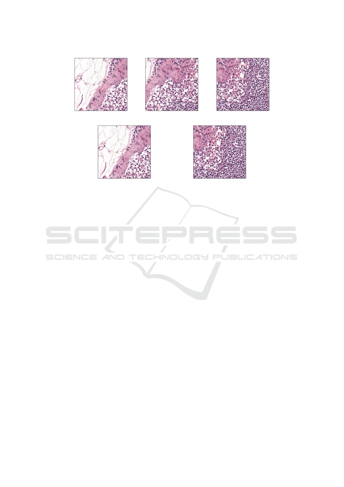
Figure 1. In convolutional layers, two dimensional

ﬁlters are applied to the image data to extract fea-

tures such as edges, objects, and colors. An exam-

ple of a convolution can be seen in Figure 2. These

features are used to create a feature map. Convo-

lutional layers are often paired with activation func-

tions, such as ReLU (rectiﬁed linear units), which

improve speed and performance by removing nega-

tive values after a convolution has been performed

(Krizhevsky et al., 2017; Zhang et al., 2021). The

pooling layer does downsampling which reduces the

number of parameters used while trying to maintain

the features (O’Shea and Nash, 2015; Zhang et al.,

2021). Lastly, fully connected layers take inputs re-

ceived by previous layers and connect them to activa-

tion units to produce output (Zhang et al., 2021).

2.5 CNN History

In 1989, Yann Lecun introduced LeNet-5, a convo-

lutional neural network originally designed to recog-

nize handwriting digits (LeCun et al., 1998). It be-

came one of the ﬁrst widely recognized published

convolutional neural networks due to its performance

with an error rate of 0.95% on the test set of 16x16

pixel handwriting digit images (Zhang et al., 2021;

LeCun et al., 1998). LeNet-5 was also revolution-

ary for its use of backpropagation to reconﬁgure its

own internal weights using gradient descent (LeCun

et al., 1998). In 2012, convolutional neural networks

surged in popularity after AlexNet won the ImageNet

Large Scale Visual Recognition Challenge (ILSVRC)

(Krizhevsky et al., 2017). Since then, the devel-

opment of new CNN architectures rapidly expanded

with the emergence of VGG16/VGG19 (Simonyan

and Zisserman, 2015), Resnet (He et al., 2016) and

Inception (Szegedy et al., 2015). ImageNet is a pop-

ular dataset for training and benchmarking convolu-

tional neural networks and contains millions of an-

notated natural images (Deng et al., 2009). Classi-

ﬁcation and object detection are common computer

vision tasks and are included in popular challenges

such as ILSVRC (Russakovsky et al., 2015). Con-

volutional neural networks are particularly skilled at

computer vision tasks and in turn have been applied

to a wide range of medical imaging tasks.

BIOINFORMATICS 2024 - 15th International Conference on Bioinformatics Models, Methods and Algorithms

406

01010

11110

01000

010

313

312

311

Figure 2: An example of the convolution operation. This convolution uses a 3x3 ﬁlter (center grid) on an image of size 5x5

(left grid) with a stride of 1 and padding of 0. The result of the convolution is the rightmost grid. The ﬁlter used here is an

example of a ﬁlter that detects vertical lines.

2.6 Modern CNNs

One of the most popular modern CNNs is VGG16.

The Visual Geometry Group (VGG) submitted

VGG16 to the ILSVRC in 2014. It proposed an in-

crease in CNN depth and was pretrained on the Ima-

geNet dataset. This model varied from its predeces-

sors by using stacks of smaller 3x3 receptive ﬁelds in-

stead of larger 11x11 or 7x7 receptive ﬁelds. This de-

creased the number of parameters throughout the net-

work. Small convolutions had previously been tried

but no other CNNs that used these smaller ﬁlters were

as deep as VGG16, which boasted sixteen layers as its

name suggests. The VGG were able to determine that

a larger depth increased the classiﬁcation accuracy.

VGG19 was described in the same paper as VGG16

and follows a similar architecture but with nineteen

layers as opposed to sixteen (Simonyan and Zisser-

man, 2015).

Another popular modern CNN is Inception (also

known as GoogleLeNet). This neural network com-

peted in the ILSVRC 2014 challenge and acheived

high performance. Inception implements wider lay-

ers as opposed to making the entire network deeper

with more layers (Szegedy et al., 2015). This network

depth is why Inception is often referred to as a deep

convolutional neural network, while other CNNs like

VGG16 are considered shallow. This greatly reduces

the computational cost of the network in compari-

son to other modern CNNs such as VGG16 (Szegedy

et al., 2016). Like VGG16, Inception uses many

smaller ﬁlters in place of larger ﬁlters to reduce the

number of parameters needed. Inception was also

trained on the ImageNet dataset and achieved remark-

able error rates while cutting computational costs

(Szegedy et al., 2015).

Additional modern CNNs that will be discussed in

later sections include ResNet and MobileNet. ResNet

implements residual functions to reference layer in-

put, which was shown to make optimization eas-

ier. Additionally, this allowed for increased net-

work depth with lower complexity and increased ac-

curacy (He et al., 2016). MobileNet was built to be

a lightweight deep neural network by utilizing depth-

wise separable convolutions (Howard et al., 2017).

2.7 Whole Slide Image Annotations

In whole slide imaging, there are three main anno-

tation types. These types are patch level (sometimes

called pixel level), slide level, and patient level. These

three levels are illustrated in Figure 3. Each type of

annotation can be useful for different tasks. These

annotations can also be organized into a hierarchy of

speciﬁcity.

Patch level annotation is the most speciﬁc level of

annotation for whole slide images. Patch level anno-

tations guarantee that when taking patches from WSI,

every patch is fully annotated. Examples of patch

level annotations include instances where each patch

has its own classiﬁcation label, segmentation mask,

or bounding boxes (Ciga and Martel, 2021). One

example of a segmentation mask would be when a

pathologist identiﬁes cancerous regions within a tis-

sue sample and annotates all regions or pixels con-

taining cancerous cells (Khened et al., 2021). Patch

level annotations are extremely helpful for segmenta-

tion tasks as they provide the ability for high supervi-

sion. However, these annotations are much more time

consuming than slide level annotations and therefore

are less commonly available. Often, training will be

performed at a lower annotation level such as patch

level while expecting a ﬁnal output at a higher level

such as slide level or patient level (Dimitriou et al.,

Deep Learning in Digital Breast Pathology

407

2019). Aggregation from lower to higher annotation

levels is discussed in Section 4.4.

The next level of annotation is at slide level.

Slide level annotations provide one label per whole

slide. For example, a whole slide image with a slide

level annotation may be labeled carcinoma vs non-

carcinoma (Araujo et al., 2017). Slide level annota-

tions are much less time consuming to do than pixel

level annotations and are therefore more abundant. If

looking at individual patches, as is common in WSI

analysis, it is possible for a patch to not match its slide

level annotation (Dimitriou et al., 2019; Hou et al.,

2016). This is why aggregation is needed when mov-

ing from one level during training to another at pre-

diction time.

The least speciﬁc level of annotations is patient

level. Patient level annotation is similar to slide level

annotations in that a single label/class is provided,

however, this label is provided to a patient rather than

a speciﬁc slide. Patients may have multiple images.

For example, in the CAMELYON17 dataset, each pa-

tient had 5 images (Litjens et al., 2018). Patient level

annotations mean that individual slides will not be

provided a label, but rather the patient, which means

the label applies to all slides associated with the pa-

tient. This is the least speciﬁc level of annotation be-

cause it is possible to incorrectly label a whole slide

(Dimitriou et al., 2019).

3 COMMON CHALLENGES

There are many unique challenges in pathology image

analysis when trying to apply deep learning. Solu-

tions to these challenges are the basis of many works

in the ﬁeld.

3.1 Image Size

One major issue that must be addressed when trying

to apply any type of machine learning technique to

histopathology image analysis is the size of whole

slide images. Whole slide image scans are extremely

large, typically 100,000 x 100,000 pixels each (Dim-

itriou et al., 2019). With images this large, they are

not feasible for machine learning use without modi-

ﬁcations. For example, CNNs usually perform best

with smaller images around 224 x 224 pixels in size

(Ciga et al., 2021). Image compression would cer-

tainly be helpful but also has drawbacks including re-

duced image quality and distortion of important mark-

ers. It has been shown that there is a signiﬁcant per-

formance decrease in benign vs. malignant breast

tissue classiﬁcation once compression levels increase

past 32:1 (Krupinski et al., 2012). Even if extreme

downsampling were performed, the image would re-

main too large for use in a convolutional neural net-

work (Ciga et al., 2021). A common approach to ad-

dress this issue is to split the image into smaller im-

ages that would be more suitable for use by machine

learning models (Hou et al., 2016). These methods

are discussed in Section 4.3.

3.2 Data Availability

A lack of well-annotated and publicly available

training data is a well-known problem in digital

histopathology image analysis. Even when images

are available, domain knowledge is required to anno-

tate these images to make them suitable for analysis

via machine learning methods. Researchers have a

few options: use a publicly available dataset, or cre-

ate their own, using images provided to them by an

institution or pathologist. One of the most popular

datasets used in breast histopathology image analysis

is the CAMELYON dataset, which is a publicly avail-

able dataset of whole slide images along with their

associated pathologist annotations. This dataset was

collected from Dutch hospitals and contains 1,399

unique whole slide images totaling 2.95 terabytes.

Slides were scanned with three different scanners

based on which hospital they came from, with the ma-

jority of hospitals using the 3DHistech Pannoramic

Flash II 250 while the Hamamatsu NanoZoomer-

XR C12000-01 scanner and Philips Ultrafast Scanner

were both used by one hospital each. All 1,399 WSI

were annotated with a slide level label. Additionally,

399 slides from CAMELYON16 and 50 slides from

CAMELYON17 were also annotated at the patch level

(Litjens et al., 2018).

As of the 2018 publication about the dataset,

it had already been accessed by over 1000 users.

Along with the dataset came the CAMELYON16 and

CAMELYON17 challenges, which encouraged teams

to design models to classify breast cancer metastases

(Litjens et al., 2018). Although the main goal of

the CAMELYON challenges is breast cancer metas-

tases detection, the dataset is widely used by re-

searchers interested in a variety of breast histopathol-

ogy image tasks. As of December 2023, the CAME-

LYON17 challenge website boasts 205 submissions

to the leaderboard with 1,943 total participants. The

current top 10 submissions on the leaderboard all

boast Cohen-Kappa scores of greater than .90 when

evaluated by the CAMELYON team.

BIOINFORMATICS 2024 - 15th International Conference on Bioinformatics Models, Methods and Algorithms

408

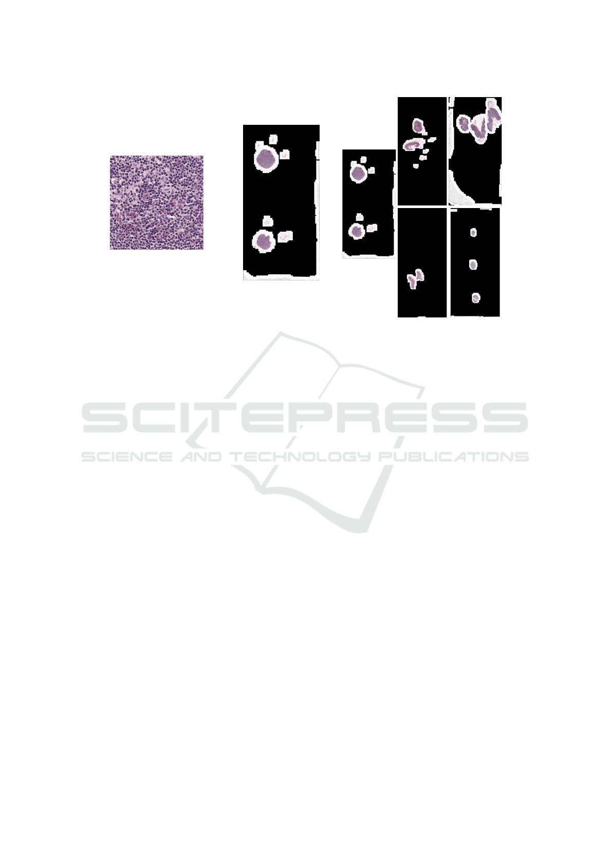
a) Image Patch b) Slide Image c) Collection of scans for a patient

Figure 3: Three main annotation types for whole slide images. (a) In patch level annotation, each image patch would have

its own classiﬁcation label or would have a pixel annotation boundary. (b) In slide level annotation, there would be a single

classiﬁcation label for the entire image. (c) In patient level annotation, there would be a single label associated with all ﬁve

images. Whole slide images come from the CAMELYON17 dataset (Litjens et al., 2018).

4 COMMON APPROACHES

4.1 Transfer Learning/Pretrained

Models

One downside to deep learning is the computational

complexity and the amount of well annotated data

needed. One technique that helps reduce model com-

plexity as well as the amount of domain speciﬁc an-

notated data needed is transfer learning (Wakili et al.,

2022). Transfer learning is another brain inspired

technique. It comes from the idea that knowledge in

one task can aid in performing a different, but some-

what related task. The use of transfer learning in con-

volutional neural networks is often used to pretrain

a CNN with large amounts of publicly available and

well annotated data, such as the ImageNet dataset.

Later, the CNN can be ﬁnetuned with domain spe-

ciﬁc data (Kim et al., 2022). Ultimately, this reduces

the amount of domain speciﬁc data needed since the

original weights will already be pretrained. Training

time is also reduced when using pretraining methods

since some portion of the training is already complete

(Gupta et al., 2022a). This is particularly useful in

ﬁelds such as digital pathology where there may be a

lack of widely available annotated data.

In a study comparing transfer learning methods in

medical imaging, Kim et al. (2022) deﬁned four types

of transfer learning based on how the training is han-

dled after the original pretraining. The feature extrac-

tor method freezes the convolutional layers and only

retrains model weights in the fully connected layers.

The feature extractor hybrid also freezes the convo-

lutional layers but replaces the fully connected layers

with another machine learning model, such as a sup-

port vector machine (SVM). The ﬁne-tuning method

unfreezes a few of the convolutional layers to be re-

trained. Finally, ﬁne tuning from scratch completely

retrains the model on the new data. After analysis of

121 publications focused on using transfer learning on

convolutional neural networks with medical images,

they recommended the feature extractor approach and

then incrementally ﬁne tuning the layers. Fine tun-

ing from scratch appeared to be a prevalent method

but did not show signiﬁcant improvements in model

accuracy despite being much more computationally

expensive than other transfer learning methods (Kim

et al., 2022).

4.2 Common Models

There are many pretrained convolutional neural net-

works available for use. Some models such as Incep-

tion have become commonly used because of their

good performance. One review of medical imaging

using CNNs found that most works use multiple mod-

els. However, Inception was the leading model when

Deep Learning in Digital Breast Pathology

409

only one model was used (Kim et al., 2022).

While tumor detection is a common task in breast

digital pathology, it is not the only task that interests

researchers. One study attempted to predict early re-

currence from histopathological images. Early recur-

rence was deﬁned as the return of a primary tumor

within three years of the original diagnosis. VGG16

pretrained on ImageNet was used in conjunction with

support vector machines (SVM). This approach ob-

served a 70.3% accuracy (67.7% sensitivity) using

within-patient validation (Shi et al., 2023). Another

study focused on predicting breast cancer recurrence

from whole slide images used six pretrained models

were used including VGG16, ResNet50, ResNet101,

Inception ResNet, EfﬁcientB5 and Xception. Two

fully connected layers were added to help reduce the

computational load. Here, Xception was found to

have the highest accuracy on the training data (91%)

and was used for further testing where it achieved an

accuracy of 87% (Phan et al., 2021).

4.3 Image Patches

Due to the enormous size of whole slide images, one

common solution is to use patches of a whole slide

image rather than the entire image itself. However,

this adds another variable, what is the optimal patch

size? There isn’t a clear-cut answer and researchers

select different patch sizes based on their speciﬁc

needs. However, some patch sizes are more often

used and are selected as default values. When select-

ing patch size, it is important to consider several fac-

tors. Finding the optimal patch size is important be-

cause it plays a role in how long training takes and can

also impact model accuracy. Patch size often depends

on the overall goal of a work. For example, works

looking to perform slide level classiﬁcation more of-

ten use larger patch sizes such as 512 x 512 and 1024

x 1024 pixels (Pinchaud, 2019; Khened et al., 2021;

Lee et al., 2021). This allows for more information to

be captured by each patch used in training and gives

a better overall view of the tissue elements and cell

architecture. However, other studies such as those fo-

cused on object detection and labeling individual cells

and nuclei, may decide to use smaller patch sizes.

Additionally, researchers need to decide whether they

will use overlapping or non-overlapping patches. An

example of the differences between overlapping and

non-overlapping patches can be found in Figure 4.

In the CAMELYON challenge there are a wide

range of approaches taken and this extends to selected

patch size. The top submission on the leaderboard for

CAMELYON17 uses a patch size of 704 x 704 pix-

els (Lee et al., 2021). However, the other submission

in the top 5 all use either 512 x 512 pixel patches,

1024 x 1024 pixel patches or some combination of

the two (Pinchaud, 2019; Khened et al., 2021; Lee

et al., 2021).

A study focusing on segmenting whole slide im-

ages from the CAMELYON dataset tried two en-

sembles with different patch sizes, 256 x 256 non-

overlapping patches and 1024 x 1024 overlapping

patches. The ensemble that used 1024 x 1024 over-

lapping patches performed slightly better than the en-

semble with 256 x 256 non-overlapping patches. This

study is currently a top 5 score on the CAMELYON17

leaderboard (Khened et al., 2021).

One work focused-on object detection of signet

ring cells. Images from 10 different organs were used,

with breast among them. Out of 127 images, each had

3 patches of size 2000 x 2000 selected for annotation

with a bounding box. A total of 12,381 signet ring

cells were annotated. However, due to overcrowd-

ing, some signet ring cells were not able to be anno-

tated. This work is also a top 5 scorer on the CAME-

LYON17 leaderboard (Li et al., 2019).

Another work used randomly selected 1000 x

1000 pixel sized patches for the task of tumor region

recognition. The patches had to be downsampled four

times to 224 x 224 to satisfy the requirements of their

selected model, MobileNetV2 (Huang et al., 2023).

There are many instances where a larger patch

size, such as 512 x 512, is initially chosen and then

cropped or resized to a smaller size like 128 x 128 to

make the image better match the selected model’s in-

put size (Phan et al., 2021). One work applied this,

originally selecting patch sizes of 512 x 512 before

randomly cropping to 448 x 448. The 448 x 448

pixel patches then went through dimension reduction

to achieve a size of 224 x 224 for training with the Ef-

ﬁcientNet framework. This study found an improve-

ment in results in both slide level classiﬁcation and

segmentation tasks with randomly cropped patches

(Ciga et al., 2021).

4.4 Annotation Aggregation

Training is often performed at a lower annotation

level such as patch level while expecting a ﬁnal out-

put at a higher level such as slide level or patient level.

In these cases, aggregation is needed to combine the

results from many patches to achieve the output for

the higher level (Dimitriou et al., 2019). One study

converted from patch level to slide level predictions

for tumor and tumor bed detections. In this case, if

one or more patches were determined to be positive

or a tumor bed was detected, the entire WSI would

be labeled as tumor positive (Ciga et al., 2021). An-

BIOINFORMATICS 2024 - 15th International Conference on Bioinformatics Models, Methods and Algorithms

410

(a)

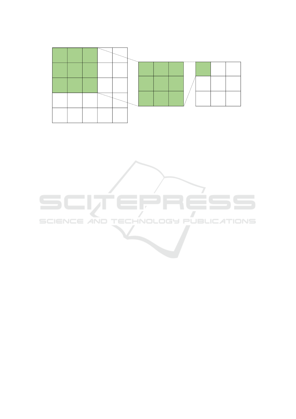
(b)

Figure 4: An example of overlapping (a) and non-overlapping (b) patches. These patches cover the same image region, but

with overlapping, three patches are needed to cover the same area as two non-overlapping patches. The ﬁrst and last patches

of (a) match the patches of (b), but the middle patch of (a) is a combination of the patches from (b). Note: these patches were

generated from whole slide images in the CAMELYON17 dataset (Litjens et al., 2018).

other study proposed a diffusion model for aggregat-

ing from patch level to slide level (Hou et al., 2016).

One study used patch level classiﬁcation to ex-

tract features for slide level classiﬁcation. 86.67% ac-

curacy was achieved using Inception for patch level

classiﬁcation. An overall accuracy of 90.43% was

achieved for the slide level classiﬁcation of normal,

benign, in situ carcinoma, and invasive carcinoma (Mi

et al., 2021).

4.5 Thresholding

When working with patches in an image, there are

hundreds of thousands of possible patches to be se-

lected depending on the patch size selected. Patch

selection methods vary between studies, with some

studies performing random patch selection while oth-

ers incorporate algorithms to select “best” patches

(Hou et al., 2016). However, one thing they all have

in common is avoiding irrelevant patches with no

cells and only background material. In most whole

slide images there are large background areas that

are irrelevant for image analysis (Veta et al., 2014).

With any patch selection technique, preprocessing

is typically performed to eliminate irrelevant back-

ground patches. Often, thresholding is used to sep-

arate the image background from the relevant mate-

rial. Thresholding is a technique that maps all im-

age pixels into one of two groups. This technique

is best used when there is high variance between an

image’s background and foreground. One popular

method of thresholding in whole slide imaging is the

Otsu thresholding technique. The Otsu threshold is

determined by ﬁnding the maximum inter-class vari-

ance (Otsu, 1979; Xu et al., 2011). While the Otsu

threshold is popular in whole slide image segmen-

tation of background and foreground, there are in-

stances where it is not as effective. For instance, in

Khened et al. (2021), the Otsu threshold could not

be used to segment the CAMELYON dataset due to

black regions within the WSI. Instead, the black pix-

els were changed to white ﬁrst and then a median blur

ﬁlter of size 7x7 kernel was used prior to performing

the Otsu thresholding. (Khened et al., 2021).

While the Otsu threshold is popular, it is not the

only thresholding method used. One study used a cus-

tom threshold to segment areas without nuclei from

the image as regions that lack nuclei are not relevant

in tumor identiﬁcation. Their thresholding removed

any regions that met the following criteria: hue be-

tween 0.5 and 0.65, saturation greater than 0.1, and

value between 0.5 and 0.9. These bounds were de-

rived from experimentation with whole slide images,

and patches with at least 25% foreground were in-

cluded in the study (Ciga et al., 2021). Neural net-

works have also been applied to the segmentation task

of tissue sample from its background with success

(Alomari et al., 2009).

Deep Learning in Digital Breast Pathology

411

4.6 Staining Techniques

Another common issue is variability in slide images.

Although hematoxylin and eosin (H&E) staining is

the most commonly used staining technique, it does

have some drawbacks. This staining technique does

not label the nuclei and cytoplasm in cells exclusively.

Sometimes other staining techniques are used such as

ﬂuorescent staining, which is more common in tis-

sue morphology clinical research. Whole slide image

datasets using H&E stained slides that are publicly

available are already scarce, so these alternative stain-

ing methods have limited annotated data to be used

for machine learning. One study attempted to bridge

H&E stained images with ﬂuorescent stained images.

Due to color variations, cross analysis can be difﬁ-

cult. Through methods involving color normaliza-

tion techniques for preprocessing and nuclei extrac-

tion, they were able to create a model that had 89.6%

accuracy in identifying tumor regions in H&E images

and 80.5% accuracy in identifying those same regions

in ﬂuorescent stained slides. Further work into cross

analysis between staining methods will increase the

amount of available data for all types of stained whole

slide image analysis (Huang et al., 2023).

4.7 Tools for Whole Slide Image

Analysis

Several approaches have produced free and open-

source software to aid others conducting research in

this area. One available tool is DigiPathAI. This

is a generalized deep learning-based framework for

histopathology tissue analysis. When creating Digi-

PathAI, four main problems were addressed – the

large size of WSI images, minimal training sam-

ples, stain variability and extraction of clinically rel-

evant features. Four datasets were used in train-

ing the model including CAMELYON16 and CAME-

LYON17 along with DigestPath (colon) and PAIP

(liver). DigiPathAI used an ensemble of 3 fully con-

volutional networks – Deeplabv3, Inception-ResNet

and DenseNet. A divide and conquer approach was

taken for the WSI image size problem. Patches of the

image were selected and segmented. Once all patches

were segmented, they stitched together the segments

to generate the whole slide image segmentation. The

researchers used data augmentation to combat a lower

number of training samples as well as to generalize

across different staining and scanning protocols. This

included horizontal/vertical ﬂip, rotations, and Gaus-

sian blurring and color augmentation (Khened et al.,

2021).

MIA (Microscopic Image Analyzer) is another

open-source tool developed for deep learning on mi-

croscopic images. MIA provides a graphical user

interface for using deep learning tools for classiﬁ-

cation, segmentation, and object detection of micro-

scopic images. By providing the graphical user in-

terface, programming skills are not required to work

with MIA. MIA simply requires training data, al-

though the user needs to be able to select a model and

hyperparameters. MIA also provides image labeling

tools for annotating datasets (K

orber, 2023).

The creators of the CAMELYON dataset also have

created an open-source tool for visualizing and in-

teracting with the CAMELYON dataset. This tool

is called ASAP (Automated Slide Analysis Platform)

and works on Linux and Windows operating systems.

ASAP offers tools for both viewing and annotation

(Litjens et al., 2018).

4.8 Comparing Machine Learning

Approaches to Pathologist Analysis

In 2017, a study put pathologists and coding teams up

to the CAMELYON16 challenge. They split pathol-

ogists into two groups and provided them with the

same WSI images for two tasks – metastases identi-

ﬁcation through pixel level annotation and slide level

labeling of metastases. 129 WSI were provided for

annotation. The ﬁrst group of pathologists was given

a time constraint of two hours while the second group

had no time constraint. The group without time con-

straint took approximately 30 hours to assess all 129

images. The challenge was open to coding teams and

32 total algorithms were submitted across 23 teams.

Of the 32 algorithms, 25 were based on deep con-

volutional nueral networks, showing their popularity

for whole slide imaging tasks. GoogleLeNet team

scored 0.994 AUC on the image classiﬁcation task. In

comparison, the median AUC for pathologists with-

out time constraint was 0.966 and 0.81 for patholo-

gists with time constraint. This showed that the model

outperformed pathologists with time constraint. This

is more realistic since pathologists have many cases

to analyze and a limited amount of time. The al-

gorithm was comparable to the results achieved by

human pathologists with unlimited time to view and

classify whole slide imaging (Bejnordi et al., ). Im-

portantly, while not perfect, CNNs can be used to pre-

dict the phenotype of breast cancers, potentially re-

ducing the need for expensive biomarker assays (Cou-

ture et al., 2018; Su et al., 2023). Deep learning algo-

rithms also have the potential to predict patient out-

come, which is hard to achieve with pathologic evalu-

ation of a breast cancer tissue sample (Shi et al., 2023;

Fernandez et al., 2022).

BIOINFORMATICS 2024 - 15th International Conference on Bioinformatics Models, Methods and Algorithms

412

5 CONCLUSION

Since the advent of whole slide imaging, research in

digital pathology has surged. Computer-aided diag-

nosis and medical image analysis have become a fo-

cus for researchers, especially in digital pathology.

While there are still many challenges when work-

ing with whole slide images, current research shows

promise for ﬁnding the solutions to overcome these

challenges. Deep learning in digital pathology has the

potential to become a powerful tool for pathologists

and assist them with the high demand of the ﬁeld,

which could ultimately lead to better care for breast

cancer patients. This paper provides background in-

formation about breast cancer, whole slide images,

and deep learning along with key challenges and the

techniques employed by researchers in the ﬁeld to

overcome these challenges. The implementation of

deep learning shows potential for incredible beneﬁts

that can both propel digital pathology forward as well

as help patients.

REFERENCES

Camelyon17 - grand challenge. https://camelyon17.

grand-challenge.org/Home/. Accessed: 2023-11-27.

Alkabban, F. M. and Ferguson, T. (2020). Breast cancer. In

StatPearls. Treasure Island (FL):Stat Pearls Publish-

ing.

Alomari, R. S., Allen, R., Sabata, B., and Chaudhary, V.

(2009). Localization of tissues in high-resolution dig-

ital anatomic pathology images. In Medical Imaging

2009: Computer-Aided Diagnosis, volume 7260.

Araujo, T., Aresta, G., Castro, E., Rouco, J., Aguiar, P.,

Eloy, C., ..., and Campilho, A. (2017). Classiﬁcation

of breast cancer histology images using convolutional

neural networks. PLoS ONE, 12(6).

Bancroft, J. D. and Layton, C. (2019). 10 - the hematoxylins

and eosin. In Suvarna, S. K., Layton, C., and Bancroft,

J. D., editors, Bancroft’s Theory and Practice of His-

tological Techniques, volume 1, pages 126–138. Else-

vier, eighth edition edition.

Bejnordi, B. E., Paul, M. V., Diest, J. V., Ginneken, B. V.,

Karssemeijer, N., Litjens, G., ..., and Ven

ancio, R.

Bhushan, A., Gonsalves, A., and Menon, J. U. (2021). Cur-

rent state of breast cancer diagnosis, treatment, and

theranostics. Pharmaceutics, 13(5).

Chan, J. K. (2014). The wonderful colors of the

hematoxylin-eosin stain in diagnostic surgical pathol-

ogy. International Journal of Surgical Pathology,

22(1):12–32.

Ciga, O. and Martel, A. L. (2021). Learning to segment im-

ages with classiﬁcation labels. Medical Image Analy-

sis, 68.

Ciga, O., Xu, T., Nofech-Mozes, S., Noy, S., Lu, F. I., and

Martel, A. L. (2021). Overcoming the limitations of

patch-based learning to detect cancer in whole slide

images. Scientiﬁc reports, 11.

Couture, H. D., Williams, L. A., Geradts, J., Nyante, S. J.,

Butler, E. N., Marron, J. S., ..., and Niethammer, M.

(2018). Image analysis with deep learning to predict

breast cancer grade, er status, histologic subtype, and

intrinsic subtype. npj Breast Cancer, 4.

Deng, J., Dong, W., Socher, R., Li, L.-J., Li, K., and Fei-

Fei, L. (2009). Imagenet: A large-scale hierarchical

image database. In IEEE Conference on Computer

Vision and Pattern Recognition.

Dimitriou, N., Arandjelovi

c, O., and Caie, P. D. (2019).

Deep learning for whole slide image analysis: An

overview. Frontiers in Medicine, 6.

Fernandez, G., Prastawa, M., Madduri, A. S., Scott, R.,

Marami, B., Shpalensky, N., ..., and Donovan, M. J.

(2022). Development and validation of an ai-enabled

digital breast cancer assay to predict early-stage breast

cancer recurrence within 6 years. Breast Cancer Re-

search, 24.

Gupta, J., Pathak, S., and Kumar, G. (2022a). Deep learn-

ing (cnn) and transfer learning: A review. Journal of

Physics: Conference Series, 2273(1):012029.

Gupta, V., Mishra, V. K., Singhal, P., and Kumar, A.

(2022b). An overview of supervised machine learning

algorithm. In 2022 11th International Conference on

System Modeling & Advancement in Research Trends

(SMART).

He, K., Zhang, X., Ren, S., and Sun, J. (2016). Deep resid-

ual learning for image recognition. In IEEE Confer-

ence on Computer Vision and Pattern Recognition.

Hou, L., Samaras, D., Kurc, T. M., Gao, Y., Davis, J. E.,

and Saltz, J. H. (2016). Patch-based convolutional

neural network for whole slide tissue image classiﬁ-

cation. In IEEE Conference on Computer Vision and

Pattern Recognition.

Howard, A. G., Zhu, M., Chen, B., Kalenichenko, D.,

Wang, W., Weyand, T., ..., and Adam, H. (2017). Mo-

bilenets: Efﬁcient convolutional neural networks for

mobile vision applications. CoRR, abs/1704.04861.

Huang, P. W., Ouyang, H., Hsu, B. Y., Chang, Y. R.,

Lin, Y. C., ..., Y. A. C., and Pai, T. W. (2023).

Deep-learning based breast cancer detection for cross-

staining histopathology images. Heliyon, 9(2).

Khened, M., Kori, A., Rajkumar, H., Krishnamurthi, G.,

and Srinivasan, B. (2021). A generalized deep learn-

ing framework for whole-slide image segmentation

and analysis. Scientiﬁc Reports, 11.

Kim, H. E., Cosa-Linan, A., Santhanam, N., Jannesari, M.,

Maros, M. E., and Ganslandt, T. (2022). Transfer

learning for medical image classiﬁcation: a literature

review. BMC Medical Imaging, 22(1).

orber, N. (2023). Mia is an open-source standalone deep

learning application for microscopic image analysis.

Cell Reports Methods, 3(7).

Krizhevsky, A., Sutskever, I., and Hinton, G. E. (2017). Im-

agenet classiﬁcation with deep convolutional neural

networks. Communications of the ACM, 60(6).

Krupinski, E. A., Johnson, J. P., Jaw, S., Graham, A. R.,

and Weinstein, R. S. (2012). Compressing pathol-

Deep Learning in Digital Breast Pathology

413

ogy whole-slide images using a human and model ob-

server evaluation. Journal of Pathology Informatics,

3:17.

LeCun, Y., Bottou, L., Bengio, Y., and Haffner, P. (1998).

Gradient-based learning applied to document recogni-

tion. Proceedings of the IEEE, 86(11):2278–2324.

LeCun, Y., Hinton, G., and Bengio, Y. (2015). Deep learn-

ing. Nature, 521:436–444.

Lee, S., Cho, J., and Kim, S. W. (2021). Automatic classiﬁ-

cation on patient-level breast cancer metastases.

LeNail, A. (2019). Nn-svg: Publication-ready neural net-

work architecture schematics. Journal of Open Source

Software, 4(33):747.

Li, J., Yang, S., Huang, X., Da, Q., Yang, X., ..., Z. H.,

and Li, H. (2019). Signet ring cell detection with a

semi-supervised learning framework. In Information

Processing in Medical Imaging, volume 11492, pages

842–854.

Litjens, G., Bandi, P., Bejnordi, B. E., Geessink, O., Balken-

hol, M., Bult, P., ..., and van der Laak, J. (2018). 1399

h&e-stained sentinel lymph node sections of breast

cancer patients: The camelyon dataset. GigaScience,

7(6).

Mi, W., Li, J., Guo, Y., Ren, X., Liang, Z., Zhang, T., and

Zou, H. (2021). Deep learning-based multi-class clas-

siﬁcation of breast digital pathology images. Cancer

Management and Research, 13.

Nounou, M. I., ElAmrawy, F., Ahmed, N., Abdelraouf, K.,

Goda, S., and Syed-Sha-Qhattal, H. (2015). Breast

cancer: Conventional diagnosis and treatment modal-

ities and recent patents and technologies. Breast Can-

cer: Basic and Clinical Research, 9s2.

O’Shea, K. and Nash, R. (2015). An introduction to convo-

lutional neural networks. ArXiv e-prints, 10.

Otsu, N. (1979). Threshold selection method from gray-

level histograms. IEEE Transactions on Systems,

Man, and Cybernetics, 9(1):62–66.

Pantanowitz, L., Farahani, N., and Parwani, A. (2015).

Whole slide imaging in pathology: advantages, lim-

itations, and emerging perspectives. Pathology and

Laboratory Medicine International, 7:23–33.

Phan, N. N., Hsu, C. Y., Huang, C. C., Tseng, L. M., and

Chuang, E. Y. (2021). Prediction of breast cancer re-

currence using a deep convolutional neural network

without region-of-interest labeling. Frontiers in On-

cology, 11.

Pinchaud, N. (2019). Camelyon17 challenge.

Pouyanfar, S., Sadiq, S., Yan, Y., Tian, H., Tao, Y., Reyes,

M. P., ..., and Iyengar, S. S. (2018). A survey on

deep learning: Algorithms, techniques, and applica-

tions. ACM Computing Surveys, 51(5):1–36.

Russakovsky, O., Deng, J., Su, H., Krause, J., Satheesh,

S., Ma, S., ..., and Fei-Fei, L. (2015). Imagenet large

scale visual recognition challenge. International Jour-

nal of Computer Vision, 115:211–252.

Sari, C. T. and Gunduz-Demir, C. (2019). Unsupervised

feature extraction via deep learning for histopatholog-

ical classiﬁcation of colon tissue images. IEEE Trans-

actions on Medical Imaging, 38(5):1139–1149.

Shi, Y., Olsson, L. T., Hoadley, K. A., Calhoun, B. C.,

Marron, J. S., Geradts, J., ..., and Troester, M. A.

(2023). Predicting early breast cancer recurrence from

histopathological images in the carolina breast cancer

study. npj Breast Cancer, 9:92.

Siegel, R. L., Miller, K. D., Wagle, N. S., and Jemal, A.

(2023). Cancer statistics, 2023. CA: A Cancer Journal

for Clinicians, 73(1):17–48.

Simonyan, K. and Zisserman, A. (2015). Very deep convo-

lutional networks for large-scale image recognition. In

ICLR.

Su, Z., Niazi, M. K. K., Tavolara, T. E., Niu, S., Tozbikian,

G. H., Wesolowski, R., and Gurcan, M. N. (2023).

Bcr-net: A deep learning framework to predict breast

cancer recurrence from histopathology images. PLoS

ONE, 18(4).

Szegedy, C., Liu, W., Jia, Y., Sermanet, P., Reed, S.,

Anguelov, D., ..., and Rabinovich, A. (2015). Go-

ing deeper with convolutions. In IEEE Conference on

Computer Vision and Pattern Recognition.

Szegedy, C., Vanhoucke, V., Ioffe, S., Shlens, J., and Wojna,

Z. (2016). Rethinking the inception architecture for

computer vision. In IEEE Conference on Computer

Vision and Pattern Recognition, pages 2818–2826.

Veta, M., Pluim, J. P., Diest, P. J. V., and Viergever, M. A.

(2014). Breast cancer histopathology image analysis:

A review. IEEE Transactions on Biomedical Engi-

neering, 61(5):1400–1411.

Wakili, M. A., Shehu, H. A., Sharif, M. H., Sharif, M.

H. U., Umar, A., Kusetogullari, H., ..., and Uyaver,

S. (2022). Classiﬁcation of breast cancer histopatho-

logical images using densenet and transfer learning.

Computational Intelligence and Neuroscience, 2022.

Watkins, E. J. (2019). Overview of breast cancer. Jour-

nal of the American Academy of Physician Assistants,

32(10):13–17.

Xu, X., Xu, S., Jin, L., and Song, E. (2011). Characteristic

analysis of otsu threshold and its applications. Pattern

Recognition Letters, 32(7).

Zarella, M. D., Bowman, D., Aeffner, F., Farahani, N.,

Xthona, A., Absar, S. F., ..., and Hartman, D. J. (2019).

A practical guide to whole slide imaging a white pa-

per from the digital pathology association. Archives of

Pathology & Laboratory Medicine, 143:222–234.

Zhang, A., Lipton, Z. C., Li, M., and Smola, A. J. (2021).

Dive into Deep Learning. Cambridge University

Press. https://D2L.ai.

BIOINFORMATICS 2024 - 15th International Conference on Bioinformatics Models, Methods and Algorithms

414