Pseudo-Curvature of Fractal Curves for Geometric Control of Roughness

Mohamad Janbein

, Christian Gentil

, C

eline Roudet

and Clement Poull

Laboratoire d’Informatique de Bourgogne (LIB), Universit

e de Bourgogne, 9 Av. Alain Savary, 21000 Dijon, France

Keywords:

Curve, Fractal Geometry, Iterated Function System (IFS), Nowhere Differentiability, Tangent, Curvature.

Abstract:

Fractal geometry is a valuable formalism for synthesizing and analyzing irregular curves to simulate non-

smooth geometry or roughness. Understanding and controlling these geometries remains challenging because

of the complexity of their shapes. This study focuses on the curvature of fractal curves deﬁned from an Iter-

ated Function System (a set of contractive operators). We introduce the Differential Characteristic Function

(DCF), a new tool for characterizing and analyzing their differential behavior. We associate a family of DCF

to the ﬁxed point of each operator. For each dyadic point of the curve, there exist left and right families of DCF

inducing left and right ranges of curvatures: the pseudo-curvatures. A set of illustrations shows the inﬂuence

of these pseudo-curvatures on the geometry of fractal curves. We propose a ﬁrst approach for applying our

results to roughness generation and control.

1 INTRODUCTION

Rough curves and surfaces have gained prominence

in ﬁelds like quality control, computer-aided design,

and computer graphics. They are utilized for di-

verse applications such as generating coherent ter-

rains (Fournier et al., 1982; Warszawski et al., 2019),

creating textures (Wang et al., 2021), or simulating

their effects to replicate the light-matter interactions

(Stam, 2001; Walter et al., 2007; Chermain et al.,

2021) without adding geometric complexity.

There are different ways to produce roughness. In

mathematics, roughness denotes irregularity in non-

differentiable context. Quantifying such irregularity

is established using mathematical constructs, like the

Lipschitz coefﬁcient and the H

older coefﬁcient in its

various forms, pointwise, local, or global. Rough

curves were ﬁrst introduced by Bolzano (Bolzano,

1851; Thim, 2003), Weierstrass (Hardy, 1916) and

Takagi (Allaart and Kawamura, 2012; Allaart and

Kawamura, 2010). They follow an iterative construc-

tion, creating new details with decreasing amplitude

related to the increasing frequency. This construc-

tion process results in a self-similar property related

to fractal geometry (Mandelbrot, 1977), and fractal

dimensions (Nayak et al., 2019). Another approach

https://orcid.org/0000-0003-3271-0712

https://orcid.org/0000-0002-0343-3456

https://orcid.org/0000-0002-0704-081X

https://orcid.org/0000-0002-4402-2928

to producing rough phenomena is to use statistical

models. For example, the pioneer Perlin noise (Per-

lin, 1985) can produce rough-looking constructs with

a high enough octave. However, many of these proce-

dural noise models lack global control.

Designing and controlling the geometry of rough

curves and surfaces is challenging. This paper aims to

enrich the understanding of differential properties of

fractal curves by studying curvature to provide tools

for later designing and controlling rough curves and

surfaces. Roughness is characterized by irregulari-

ties (differential behavior), often associated with self-

similarity. Consequently, fractals offer an appropriate

framework for studying phenomena related to rough-

ness and irregularity. Deterministic is also essen-

tial for accurate controls and continuous dependency

between parameters and resulting geometry. Conse-

quently, we focus on fractal deterministic curves.

We review some related work in section 2. We

focus on deterministic fractal curves deﬁned by Iter-

ated Function Systems (IFS) (Hutchinson, 1981) and

projected IFS, as explained in section 3. Section 4

introduces the differential characteristic function, a

new tool to analyze the differential behavior of fractal

curves. Section 5 shows how the differential char-

acteristic functions can be used to obtain known re-

sults about the tangent of a fractal curve. In section 6,

we analyze the curvature at each ﬁxed point from its

associated family of differential characteristic func-

tions, and we deﬁne the pseudo curvature of a fractal

Janbein, M., Gentil, C., Roudet, C. and Poull, C.

Pseudo-Curvature of Fractal Curves for Geometric Control of Roughness.

DOI: 10.5220/0012574800003660

Paper published under CC license (CC BY-NC-ND 4.0)

In Proceedings of the 19th International Joint Conference on Computer Vision, Imaging and Computer Graphics Theory and Applications (VISIGRAPP 2024) - Volume 1: GRAPP, HUCAPP

and IVAPP, pages 177-188

ISBN: 978-989-758-679-8; ISSN: 2184-4321

177

curve. Finally section 7 discusses applying our results

to roughness design and generation.

2 RELATED WORK

The automatic generation (for our purpose, geome-

tries) implies having speciﬁcations, generally ex-

pressed in terms of expected properties or characteris-

tic values. Of course, these speciﬁcations have to de-

pend on the generator parameters. The nature of this

dependency and its accessibility are central to having

an intuitive control or facilitating the speciﬁcation de-

scription.

Numerous studies deal with this question using

spectral analysis to generate noises (fractal-based,

colored noises, convolution noise) (Perlin, 1985;

Cook and DeRose, 2005; Lagae et al., 2009; Gilet

et al., 2014; Pavie, 2016; Cavalier et al., 2019; Hu

and Tonder, 1992; Wang et al., 2021; P

erez-R

afols

and Almqvist, 2019). However, most need spec-

tral control, which is only apparent with minimum

knowledge. Other studies focus on the differential

properties of random rough curves. In tribology, the

contact area between two rough surfaces is analyzed

from the curvature. Nowicki (Nowicki, 1985) lists

and discusses numerous parameters for evaluating,

analyzing, and modeling surface roughness. Some

were concerned about differential properties like peak

shapes, slope means, number of inﬂection points, and

RMS of the proﬁle slope, radius of asperity, and cur-

vature radius. However, he only provides standard

deﬁnitions for smooth curves without considering the

numerical trouble caused by the irregularity of rough

curves. Moalic et al. (Moalic et al., 1987) outline

errors arising in the computation of slopes and cur-

vatures statistical characteristics (mean, variance) for

actual sampled surface. The tested methods by or-

der of decreasing error are the ﬁnite difference meth-

ods (Whitehouse, 1982), the autospectrum approach,

and the Fourier transform computation. However, all

these methods evaluate the characteristics on aver-

age. Bigerelle et al. (Bigerelle et al., 2013) propose

a method to calculate the curvature at any point of

a random rough curve by considering the statistical

self-similarity (fractal) property.

To eliminate the uncertainty of the randomness,

some authors focus on deterministic curves. Daoudi

et al. (Daoudi et al., 1998) construct nowhere dif-

ferentiable continuous functions from prescribed lo-

cal H

older regularity at each point. However, the

older irregularity is a complex notion. Bensoudane

and Podokorytov (Bensoudane et al., 2009; Podkory-

tov, 2013) focus on curves built with IFS and show

that it is possible to deﬁne left and right tangents even

if the curve is nowhere differentiable. In some conﬁg-

urations, tangents are not deﬁned, but the differential

behavior is described by deﬁning pseudo-tangents.

These studies have shown accuracy brought by deter-

ministic models. Pseudo-tangents are an interesting

geometric tool for controlling roughness, but they are

insufﬁcient to manage the complexity of such curves.

A second-order differential characteristic is expected.

3 BACKGROUND

An Iterated Function System (IFS) is a ﬁnite set of

contractive operators

{

}

I−1

i=0

that act on a complete

metric space (X,d). For a given IFS, there exists

a unique non-empty compact set A of (X,d) satis-

fying the self-similarity property: A =

I−1

i=0

(A).

Note that each operator T

maps A onto a part of it-

self. A is called the attractor of the IFS. We com-

pute it using the Hutchinson operator T, deﬁned by

T(K) =

I−1

i=0

(K), with K ∈ H(X), the set of all

non-empty compact subsets of X. The attractor A can

be obtained as the limit of an iterative process, given

by A = lim

i→+∞

(A).

Zair and Tosan (Zair and Tosan, 1996) and

Schaefer (Schaefer et al., 2005) introduced the pro-

jected IFS model to create free-form fractal shapes

that can be deformed by changing the positions

of a set of N control points P = {P

,.. .,P

N−1

The attractor is deﬁned in the barycentric space

α ∈ R

∑

N−1

j=0

= 1,α = (α

,...,α

N−1

)

(Figure 1 left). Each point of A ⊂ BI

is inter-

preted as a set of weights w.r.t. the control points.

The attractor is then projected onto the modeling

space according to a set of control points P: PA =

p ∈ X, p =

∑

N−1

j=0

: α ∈ A

(see Figure 1 right).

This construction is similar to B

ezier curves deﬁ-

nition, where the Bernstein polynomial functions are

deﬁned in BI

and then projected according to the

set of control points: C(t) =

∑

N−1

j=0

(t)P

. Note that

ezier (resp. NURBS) curves can be modeled using

projected IFS (Zair and Tosan, 1996) (resp. C-IFS

(Morlet et al., 2019)).

For the rest of the paper, all operators are con-

tractive afﬁne operators acting on BI

. We consider

the barycentric space BI

as an hyperplane of the

afﬁne space R

, with the coordinate system of ori-

gin O = (0, ... ,0) and basis vectors (e

,.. .,e

N−1

)

where the j

component of the N-dimensional vector

)

= δ

i j

, where δ

i j

designates the Kronecker delta.

The associated vector space of BI

is the set of vec-

GRAPP 2024 - 19th International Conference on Computer Graphics Theory and Applications

178

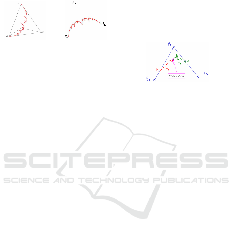
Figure 1: Left: Takagi attractor A built in the barycentric

space BI

, where {e

} are the canonical basis vec-

tors. Right: projection of the attractor A of the left ﬁgure

according to the set of control points

{

}

tors BI

v ∈ R

∑

N−1

j=0

= 0

. Consider an IFS

{

}

I−1

i=0

, for each operator T

: BI

→ BI

, there ex-

ists a linear operator T

: BI

→ BI

such that:

(x + v) = T

(x) + T

(v) (1)

for any x ∈ BI

and any v ∈ BI

. Each operator T

must be internal (a point of BI

is mapped onto BI

As a consequence, their matrix form, expressed in the

coordinate system (O,e

,.. .,e

N−1

), are N × N matri-

ces with column’s sum equals 1 (T

have the same

matrix form as T

). Because of the constraint on the

sum of each column, such matrices have 1 as eigen-

value. To be contractive, the remaining eigenvalues

must have their modulus lesser than 1. For an opera-

tor T

, we adopt the following notation for its eigen-

values and eigenvectors: (λ

= 1,λ

,.. .,λ

N−1

) and

,.. .,v

N−1

), respectively, where eigenvalues are

arranged in decreasing modulus (upper index). The

ﬁrst eigenvector v

(not in bold), associated to λ

= 1,

corresponds to the ﬁxed point, denoted by c

. The

sum of its components equals 1, meaning it is a point

of BI

. The other eigenvectors have the sum of their

coordinates equal to zero, indicating that these eigen-

vectors are vectors. For example, we can consider the

matrices of de Casteljau, which are used in the calcu-

lation of B

ezier curves:





1 1/2 1/4

0 1/2 1/2

0 0 1/4





, T





1/4 0 0

1/2 1/2 0

1/4 1/2 1





The attractor of the associated IFS is the Bernstein poly-

nomial function of degree 2 lying in BI

With projected IFS, controlling the topology of such

objects is challenging. An extension, named Boundary

Controlled Iterated Function System (BC-IFS) (Sokolov

et al., 2015; Gentil et al., 2021), provides a control of

the attractor topology with incidence and adjacency con-

straints. Ensuring the C

(0)

continuity for curves is equiv-

alent to applying the well-known constraints for Fractal

Interpolation Functions (FIF) (Barnsley, 2014). We con-

sider an IFS composed of two operators T

and T

that

builds an attractor in BI

(as in Figure 2). The attrac-

tor is then projected onto the modeling space using three

control points {P

} deﬁned in R

. The operator

maps all the curve to the red part of the curve, and T

maps it into the green part, so to guarantee that the two

parts are connected, we impose the adjacency constraint

for C

(0)

: T

= T

, where the ﬁxed points c

and c

are the left and right endpoints of the curve respectively

(see Figure 2).

Figure 2: Adjacency constraint for C

(0)

continuity: T

is imposed for the IFS composed of T

and T

to guar-

antee the connectivity of the fractal curve at the joining

point, the curve is then projected into the modeling space

with control points

{

}

We deﬁne dyadic points, on which we compute the

pseudo-curvature as following: p ∈ A is a dyadic point

if there exists a ﬁnite sequence of indices σ

,σ

,...,σ

(where σ

∈ {0, ...,I − 1} and σ

l−1

̸= σ

) s.t. p =

...T

l−1

4 CHARACTERIZATION OF

ITERATIVE BEHAVIORS

The main idea of this paper is to consider an attractor as a

set of sequences. We know that each T

has a ﬁxed point

belonging to the attractor. By applying T

iteratively

on the ﬁxed point c

of another operator T

, we deﬁne a

sequence of points converging to c

, each element of the

sequence belonging to the attractor.

This section introduces the differential characteris-

tic function (DCF) to formalize and simplify these se-

quences’ behavior.

4.1 Elementary Iterative Behavior of

One Operator

Consider an internal contractive operator T (of an IFS

deﬁning a curve) acting on BI

, (λ

= 1,λ

,λ

) its eigen-

values, (v

= c, v

) its eigenvectors and q

a point of

We deﬁne the sequence {q

}

n∈N

by: q

= T

. Each

term of this resulting sequence can be expressed in the

coordinate system {c,v

= c + x

+ x

, where x

∈ R (2)

= T

c + T

+ x

) (3)

= c + x

(λ

)

+ x

(λ

)

(4)

Pseudo-Curvature of Fractal Curves for Geometric Control of Roughness

179

To gain insight into the differential properties of the

curve, we need to analyze the different behaviors of

the sequence {q

}

n∈N

w.r.t. the eigensystem of T . To

see clearly these behaviors, we project the sequence of

points T

onto the modeling space in a way to have

an orthogonal system {Pc, Pv

,Pv

} such that ||Pv

|| =

||Pv

|| and then ||Pλ

|| and ||Pλ

|| reﬂect the value

of the eigenvalues (as shown in the ﬁgures below). The

different cases are deﬁned from the eigenvalues:

• Case 1: if λ

> λ

> 0, the contraction in the direc-

tion of v

is greater than that in the direction of v

the sequence converges to the point Pc tangentially

to the eigenvector v

. Figure 3 left illustrates the dif-

ferent conﬁgurations according to the location of the

starting point in the four quadrants deﬁned from the

eigenvectors.

• Case 2: if |λ

| > |λ

|, λ

< 0 and λ

< 0, the com-

ponents x

(λ

)

and x

(λ

)

of q

alternates between

positive and negative values as a function of n, and

therefore the sequence of points passes alternately

from the starting quadrant to the opposite one (Fig-

ure 3 right).

Figure 3: Left: Applying T (with eigenvalues λ

> λ

) on

four different starting points (Pq

,Pq

′

,Pq

′′

,Pq

′′′

). Each se-

quence converges to Pc tangentially to Pv

. Right: λ

< 0

and λ

< 0: the sequence of points {PT

}

n∈N

alternates

between the starting quadrant to the opposite one until con-

verging towards the point Pc.

• Case 3: if |λ

| > λ

> 0 and λ

< 0, the component

(λ

)

of q

alternates between positive and nega-

tive values as a function of n, and therefore the se-

quence of points passes alternately from one of the

half-planes delimited by the line c +tv

to the other

half-plane (Figure 4 left).

• Case 4: if λ

> |λ

| and λ

< 0, the component

(λ

)

of q

alternates between positive and neg-

ative values as a function of n, and therefore the se-

quence of points passes alternately from one of the

half-planes delimited by the line c +tv

to the other

half-plane. But the sequence already converges to c

tangentially to v

(Figure 4 right).

• Case 5: λ

= λ

> 0, the contractions in the direc-

tions of v

and v

are equal, and the sequence of

points converges on a straight line to the point Pc.

• Case 6: if λ

are complex eigenvalues, the oper-

ator is characterized by a rotation, and the sequence

of points converges on a spiral to the point Pc.

Figure 4: In both ﬁgures, the sequences of points

{PT

}

n∈N

converge to the point Pc. They alternate be-

tween the positive and negative half-planes delimited by the

second eigenvector Pλ

(for the left ﬁgure, where λ

< 0)

or by the ﬁrst one Pλ

(for the right ﬁgure, where λ

< 0).

4.2 The Differential Characteristic

Function

In order to analyze the differential properties at the ﬁxed

point c of a contractive operator T , we aim to ﬁnd an

analytical function that interpolates the points of the se-

quence obtained by applying T on a starting point q

This expression will allow a formal characterization of

the differential behavior at the limit point of the se-

quence.

We ﬁrst focus on the simplest case with T acting on

and where both λ

and λ

are positive (i.e. 1 > λ

> 0). We will present the other conﬁgurations later.

Deﬁnition. Consider an operator T acting on BI

with

eigenvalues (λ

= 1 > λ

> λ

> 0) and associated

eigenvectors (v

= c, v

). We suppose v

and v

in-

dependent. Let q be a point of BI

\{c + tv

}

t∈R

(i.e. q

does not belong to the line passing through c in the direc-

tion of v

), and consider its expression in the coordinates

system (c, v

): q = c + x

+ x

. We suppose that

and v

are chosen such that x

> 0 and x

> 0. The

differential characteristic function (DCF) is deﬁned by:

T,q

(t) = c + tv

+ βt

, t ∈ R

(5)

where β =

)

and α =

log(λ

)

log(λ

)

Property. D

T,q

interpolates the points of the sequence

{

}

n∈N

{

}

n∈N

(see Figure 5 left).

Proof. q

= c + x

+ x

, where x

∈ R

+∗

= T

= c + x

(λ

)

+ x

(λ

)

= c + X

+ X

We have to prove that q

have their coordinates

) in the form (t,βt

). Set t = X

= x

(λ

)

then:

βt

= β(x

(λ

)

((λ

)

. Because α =

log(λ

)

log(λ

)

, λ

= (λ

)

, x

(λ

)

= βt

and X

= βt

Property. The graph of D

T,q

(t), denoted by

Graph(D

T,q

), is invariant under T .

Proof. Consider a DCF D

T,q

(t) = c+tv

+βt

. Let m

be a point of Graph(D

T,q

), m = c + t

+ βt

. Then

T m = c + λ

+ λ

βt

and as λ

= (λ

)

, T m =

c + λ

+ β(λ

)

∈ Graph(D

T,q

)

GRAPP 2024 - 19th International Conference on Computer Graphics Theory and Applications

180

Remark. If s ̸∈ Graph(D

T,q

), then β

̸= β, and D

T,s

different from D

T,q

(see Figure 5 right).

Figure 5: Various DCFs D

T,q

(t) = c +tv

+βt

with dif-

ferent starting points (q

, m or s). In the right ﬁgure, D

T,q

(in red) interpolates both green and red sequences of points

{PT

}

n∈N

and {PT

n∈N

(with m ∈ Graph(D

T,q

)).

In blue, D

T,s

(s ̸∈ Graph(D

T,q

)) interpolates the blue se-

quence of points.

In the deﬁnition of the DCF, we previously imposed

conditions on λ

and λ

. We discuss here the gen-

eral conﬁguration. For the speciﬁc cases where x

are null, D

T,q

is deﬁned as follows: if x

= 0 then

T,q

(t) = c + tv

and if x

= 0 then D

T,q

(t) = c + tv

If both x

and x

are null D

T,q

is not deﬁned (q

= c the

ﬁxed point of T ). If λ

and/or λ

are strictly negative,

we deﬁne a double DCF, one interpolating the sequence

of points {PT

}

n∈N

with even values of n, and one for

odd values:

• Case 1: λ

and λ

are strictly negative (see Fig 6):

– D

T,q

(t) = c + tv

+ βt

for even values of n.

– D

T,q

(t) = c − tv

− βt

for odd values of n.

Figure 6: λ

< 0 and λ

< 0 ⇒ double DCF, the ﬁrst one in

blue interpolating the points of the sequence {PT

}

n∈N

for even indices, and the second one in green for odd in-

dices.

• Case 2: λ

strictly negative (see Fig 7 left):

– D

T,q

(t) = c + tv

+ βt

for even values of n.

– D

T,q

(t) = c − tv

+ βt

for odd values of n.

• Case 3: λ

strictly negative (see Fig 7 right):

– D

T,q

(t) = c + tv

+ βt

for even values of n.

– D

T,q

(t) = c + tv

− βt

for odd values of n.

• Case 4: λ

strictly negative and |λ

| = λ

> 0:

– D

T,q

(t) = c + tv

+ βtv

for even values of n.

– D

T,q

(t) = c − tv

+ βtv

for odd values of n.

Now, consider a fractal curve deﬁned in a barycentric

space BI

, from a set of I operators {T

}

I−1

i=0

. For a given

Figure 7: For both ﬁgures, two DCFs are shown with dif-

ferent colours. The blue one interpolates the points of the

sequence {PT

}

n∈N

with even indices, the green one for

odd indices. λ

< 0 for the left ﬁgure and λ

< 0 for the

right one.

operator T

and from each point q

of the curve, we can

deﬁne a sequence of points {q

}

n∈N

belonging to the

curve and consequently a simple or double DCF. Fig-

ure 8 shows a fractal curve in BI

deﬁned from an IFS

composed of two operators T

and T

, and projected into

the modeling space using four control points. This curve

has many points having different values of β. Applying

iteratively to these points results in many sequences

of points converging to the left endpoint c

, such as the

two sequences displayed in blue and black in the ﬁgure

with their corresponding DCFs. Let us denote the set of

Figure 8: In blue and black, the two different sequences

obtained by applying T

iteratively to Pq

and Pq

′

are con-

verging to the limit point Pc

all DCFs representing all sequences converging to c

by:

FDCF(i) = {D

∈ A} (6)

In the following section, we will analyze FDCF(i) to

characterize the differential behavior in the neighbor-

hood of c

. Then, we will propagate these results to

dyadic points thanks to the self-similarity property.

5 PSEUDO-TANGENT

PROPERTIES OF FRACTAL

CURVES USING DCF

In this section, we show how we obtain known results

given by Bensoudane et al. (Bensoudane, 2009).

Let us consider a fractal curve deﬁned in the barycen-

tric space BI

, from a set of I operators {T

}

I−1

i=0

. The dif-

ferential behavior of a sequence of points can be directly

determined from the derivative of D

. According to

the different conﬁgurations:

Pseudo-Curvature of Fractal Curves for Geometric Control of Roughness

181

• D

′

(t) = ±v

±βαt

α−1

, when x

̸= 0 and x

̸= 0,

• D

′

(t) = ±v

, when x

= 0,

• or D

′

(t) = ±v

, when x

= 0.

The tangent at t = 0 is:

• If α > 1, D

′

(0) = ±v

(if x

̸= 0) or D

′

(0) =

±v

(if x

= 0).

The derivative depends only on which quadrant q

belongs.

• If α = 1, D

′

(0) = ±v

± βv

The derivative depends on the position of q

This means that if all curve points satisfy the same con-

ditions in terms of x

and x

, all iterative sequences will

converge to the ﬁxed point with the same tangent.

Note that the tangent lies in the barycentric space.

The tangent of the projected curve according to the set

of control points is PD

′

(0) (the projection conserves

the collinearity). To have a unique behavior for all DCF

of a FDCF(i), we need to impose common constraints

on all the points of the curve. These constraints are ex-

pressed in terms of sign(x

) and/or sign(x

). To present

this analysis without ambiguity, we consider the tan-

gent itself and the direction of the ﬁnite difference at

t: ∆

[C](t) = C(t + h) −C(t), where C([0,1]) = A de-

notes the parameterised fractal curve (with C(0) = c

and C(1) = c

). In the following cases, we show differ-

ent conﬁgurations with associated example curves. Each

curve is generated by an IFS composed of two opera-

tors in BI

and then is projected into R

by a set of three

control points (black squares). We focus on T

and we

only display D

(in green). For each ﬁgure, x

and x

represents the coordinates of c

in (c

). The con-

straints on x

and x

must be satisﬁed for all q belonging

to the curve:

• Case 1: λ

> 0 and λ

> 0, x

> 0 and x

> 0 ⇒ the

tangent at Pc

is Pv

(Figure 9 left).

• Case 2: λ

< 0 and λ

< 0 ⇒ the tangent at Pc

oscillates indeﬁnitely between Pv

and −Pv

(Figure

9 right).

Figure 9: Left: the tangent at Pc

is Pv

. Right: at

, ∆

[C](0) oscillates indeﬁnitely between Pv

and −Pv

while h tends to zero.

• Case 3: λ

> 0 and λ

< 0, x

> 0 ⇒ the tangent at

is Pv

(Figure 10 left).

• Case 4: λ

< 0 and λ

> 0, x

> 0 ⇒ the tangent

at Pc

oscillates indeﬁnitely between Pv

and −Pv

(Figure 10 right).

Figure 10: Left: the tangent at Pc

is Pv

. Right: at

, ∆

[ f ](0) oscillates indeﬁnitely between Pv

and −Pv

while h tends to zero.

• Case 5: |λ

| = λ

> 0, x

> 0 ⇒ the tangent is not

deﬁned at Pc

, it oscillates indeﬁnitely between two

extrema (Figure 11).

Figure 11: In c

, ∆

[ f ](0) oscillates indeﬁnitely between

two extrema depending on the geometry of the curve, while

h tends to zero.

This analysis can be carried out on both ending

points of the curve. Then, by the self-similarity property,

each behavior is transported to the right and left sides

of each dyadic point. All possible combinations can be

obtained. In case where an eigenvalue is complex, it re-

ﬂects a rotation component in the operator, introduces a

spiral around the ﬁxed points.

6 PSEUDO-CURVATURE OF

FRACTAL CURVES

In the previous section, we showed that even if fractal

curves are generally nowhere differentiable, it is possi-

ble, with some conditions, to deﬁne right and left tan-

gents. In this section, we focus on the curvature to as-

sess the impact of the second derivative on the curve.

The curvature presents the ﬁrst advantage of being inde-

pendent of the parametrization, which is not apparent to

manage for fractal curves. Our idea is to study the cur-

vature of a fractal through the second derivative of the

FDCF.

GRAPP 2024 - 19th International Conference on Computer Graphics Theory and Applications

182

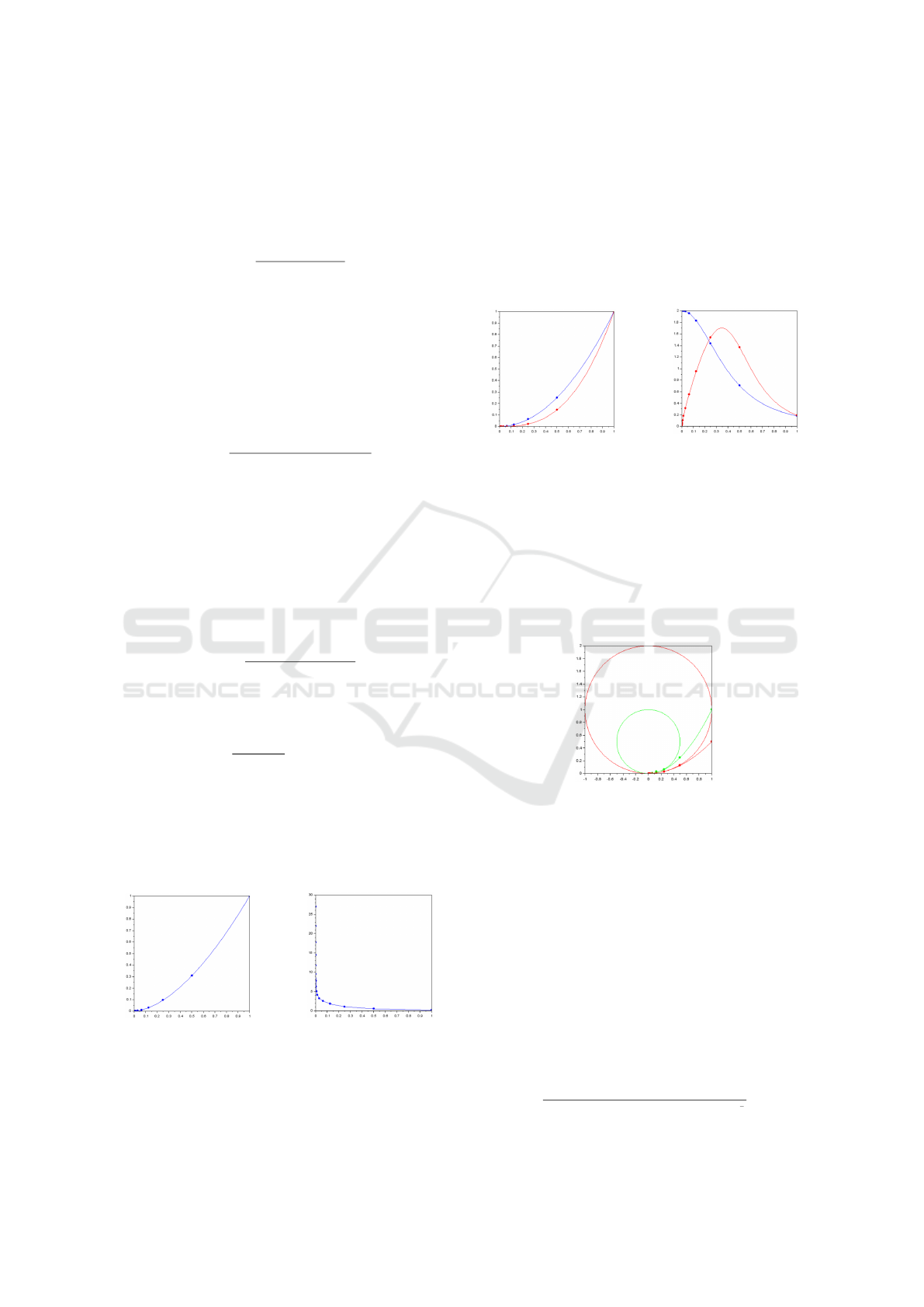
6.1 Curvature Analysis of a DCF

First, we focus on the curvature at the left and right end-

points of the curve. For a given parametric curve f (t),

the curvature κ(t) is:

κ(t) =

∥ f

′

(t) × f

′′

(t)∥

∥ f

′

(t)∥

(7)

Consider an operator T (of an IFS deﬁning a curve) act-

ing on BI

, (v

= c, v

) its eigenvectors and q

a point

of BI

. For the simplicity of calculations, we project the

sequence of points {T

}

n∈N

onto the modeling space

in a way to have an orthogonal system {Pc,Pv

,Pv

}

such that ||Pv

|| = ||Pv

|| (the general case will be given

later). From a given point q

belonging to the curve, we

can determine the curvature of PD

T,q

κ(t) =



′

T,q

(t) × PD

′′

T,q

(t)



′

T,q

(t)



(8)

Note that we compute the curvature directly in the mod-

eling space (i.e. from the projected curves) because the

cross-product has no meaning in the barycentric space.

We have:

′

T,q

(t) = Pv

+ βαt

α−1

(9)

′′

T,q

(t) = βα(α − 1)t

α−2

(10)

and Pv

are chosen orthonormal, then:

κ(t) =



βα(α − 1)t

α−2



(1 + (βαt

α−1

)

3/2

(11)

Using the tangent existence constraint: 0 < |λ

| < λ

< 1

we can deduce the domain of α:

1 <

log(|λ

log(λ

)

= α < +∞ (12)

We can distinguish three different cases for the value

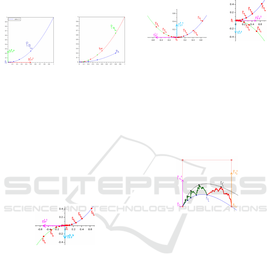
κ(t) at t = 0, depending on the value of α:

• Case 1: if 1 < α < 2 ⇒ lim

t→0

κ(t) = +∞, Figure

12 left shows in blue the curve PD

T,q

and Figure 12

right the corresponding curvature. When t tends to

zero, the curvature tends to +∞.

Figure 12: Left: the curve PD

T,q

having 1 < α < 2. Right:

the curvature values of the curve displayed on the left ﬁgure.

• Case 2: if α = 2 (λ

= λ

) ⇒ κ(0) =

2β

̸= 0. Figure

13 left shows in blue the curve PD

T,q

and Figure 13

right the corresponding curvature. When t tends to

zero, the curvature tends to a ﬁnite non-zero value

depending on β. This case induces a correspondence

between the second derivative PD

′′

T,q

and the second

eigenvector Pv

at the ﬁxed point Pc of T (PD

′′

T,q

(0)

collinear to Pv

• Case 3: if α > 2, as the curve in red (Figure 13 left)

approaches the ﬁxed point Pc, lim

t→0

κ(t) = 0 (Fig-

ure 13 right).

Figure 13: Left: in red, the curve PD

T,q

where α > 2. In

blue, the curve PD

T,q

where α = 2. Right: the correspond-

ing curvature values for the red and blue curves displayed

on the left ﬁgure.

Thanks to D

T,q

, we can characterize the differential

behavior of the sequence {q

}

n∈N

at the ﬁxed point of

an operator. In the ﬁrst and third cases, the curvature is

either zero or inﬁnite and does not depend on the value

of β. While in the case where α = 2, the curvature is

ﬁnite, non-zero and depends on the initial point q

(see

Figure 14).

Figure 14: Two starting points (on the right) having distinct

β ⇒ two distinct DCFs (curves in red and green) having

two different curvatures represented by their red and green

osculating circles at the limit point.

6.2 Curvature of a DCF in BI

and BI

In the previous section, when we have considered an op-

erator T acting on BI

, we have made the assumption

that {Pc,Pv

,Pv

} is an orthogonal system. Later, we

adapt the previous results to the general case in BI

and

after in BI

, for an IFS

{

}

Let us consider {i,j} the canonical orthonormal basis

of R

. We denote the decomposition of each projected

eigenvector of an operator T

by: Pv

= a

i + b

j for k ∈

{1,2}.

Then for each PD

(t):

κ(t)=

−b

)β

(α

−1)

−2

+2(a

)β

−1

+(a

)(β

−1

)

(13)

Pseudo-Curvature of Fractal Curves for Geometric Control of Roughness

183

From this formula and because 1 < α

log(|λ

log(λ

)

< +∞,

we have the same cases as the previous simple section:

• Case 1: 1 < α

< 2: α

− 2 < 0 then lim

t→0

κ(t) =

+∞.

• Case 2: α

= 2 then κ(0) is ﬁnite and non-zero.

The curvature at c

: κ(0) =

2β

− b

)

+ b

)

depends on β

. This case induces a correspondence

between the second derivative D

′′

and the second

eigenvector v

at c

′′

(0) collinear to v

• Case 3: α

> 2: lim

t→0

κ(t) = 0.

In general, a DCF lies in an N-dimensional barycen-

tric space BI

. Operators T

are represented by N × N

matrices, with at most N eigenvalues and N eigenvectors.

The eigenvalues have the following condition: λ

= 1 >

> |λ

| > ·· · > |λ

N−1

| > 0. Consider a starting point

= c

+· ··+x

N−1

∈ A where x

,...,x

N−1

∈

R, the DCF which interpolates the obtained sequence of

points {q

}

n∈N

(in BI

) becomes:

+tv

+β

i,2

+···+β

i,N−1

N−1

(14)

where α

i,z

log(|λ

log(λ

)

, and β

i,z

z−1

for 2 ≤ z ≤ N − 1,

and its curvature is more complex, but when t tends to

zero, most of the terms vanish, and we obtain the same

cases as for BI

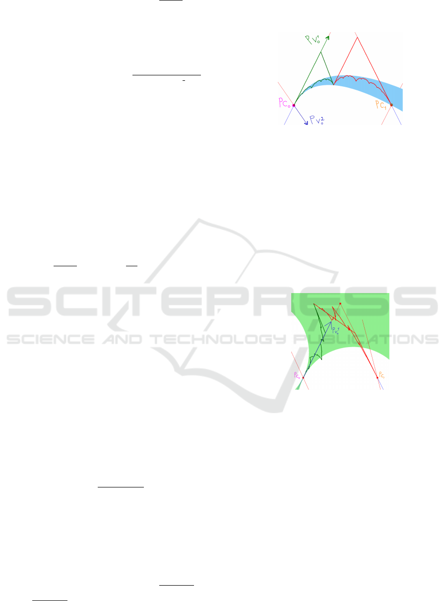
6.3 Pseudo-Curvature and FDCF

As deﬁned in section 5, we associate to each ﬁxed point

a FDCF(i). This family is deﬁned from all the points

belonging to the curve and having different values of β.

As we show in sections 6.1 and 6.2, we identify three

identical cases, depending only on α

i,2

. For cases where

1 < α

i,2

< 2 and α

i,2

> 2, the curvature doesn’t depend

on β

i,2

, meaning all DCF of FDCF(i) have the same

curvature which is inﬁnite and 0 respectively. Then we

state that the pseudo curvature of the fractal curve at c

is the common curvature of FDCF(i).

For the remaining case, where α

i,2

= 2, the curvature

is in the form:

(0) =

2β

i,2

× cst

cst

, (15)

where cst

and cst

denote two real constants. If all

points q

belonging to the fractal curve except the point

(A \ {c

}) satisfy x

> 0 and x

> 0 (implying λ

> 0

and λ

> 0), the set {β

i,2

, s.t. q

∈ A} have a lower and

an upper bound, β

i,in f

and β

i,sup

respectively. The curve

is embedded in the area deﬁned by all the graphs of

FDCF(i) as the Figure 15 shows. FDCF(i) induces a

range of curvatures bounded by κ

i,in f

2β

i,in f

×cst

cst

and

i,sup

2β

i,sup

×cst

cst

. In this case, the behavior of the curve

is too complex to be approximated by a unique circle.

We deﬁne the pseudo curvature of the fractal curve at c

by the interval [κ

i,in f

,κ

i,sup

], implying a continuous set of

osculating circles (see Figure 17).

Figure 15: In blue, the projected DCFs of FDCF(0) cover

the fractal curve.

We can observe different situations according to the

signs of λ

and λ

. For example, in Figure 16, 1 > λ

|λ

| > 0 and λ

< 0. As explained in section 3.2, con-

sidering the computation of the curvature at c

, we have

a double DCF for each sequence of points converging to

. This involves a range of curvature for both sides of

w.r.t. v

, with the same value of κ

sup

. As the curve

passes through the line c

+ tv

, there exist points s.t.

= 0 and deﬁning a DCF with a null curvature. The

pseudo-curvature is the range of curvature deﬁned from

FDCF(i) as a set of curvatures ranging in [0,κ

i,sup

] for

both sides of the line c

+tv

Figure 16: In green, we show the range of the right pseudo-

curvature at the left endpoint c

, where 0 ≤ κ ≤ 0.659 and

= −(λ

)

= −0.36.

When λ

< 0 and λ

> 0, we can do the analysis

symmetrically to the previous one. As the curve passes

through the line c

+ tv

, there exist points s.t. x

= 0

and deﬁning a DCF with the value of curvature equals

0. For both sides of the line c

+ tv

, as the point of

the curve approaches the line, the curvature of the cor-

responding DCF tends to inﬁnity. But it although exists

i,in f

as the curve is compact. The pseudo-curvature is

the range of curvature deﬁned from FDCF(i) as a set

of curvatures ranging in [κ

i,in f

,+∞[ for both sides of the

line c

+tv

and 0 on c

+tv

(see Figure 19). For dyadic

points, the pseudo-curvature can be obtained straight-

forwardly from the self-similarity property and previous

results from the endpoints of the curve. For example,

to determine the pseudo-curvature at the joining point

= T

), we just have to apply the operator T

on FDCF(1) and T

on FDCF(0) to obtain the left and

GRAPP 2024 - 19th International Conference on Computer Graphics Theory and Applications

184

the right pseudo-curvature, which is for the left pseudo-

curvature:

(t) =



′

(t) × PT

′′

(t)



′

(t)



. (16)

For the right side of the joining point, κ

(t) is deduced

from equation 16 by interchanging T

and T

. It is equiv-

alent to computing the pseudo-curvature of a new pro-

jection according to the control point P

′

= PT

. For any

dyadic point p = T

...T

l−1

we have:

(t) =



PT T

′

(t) × PT T

′′

(t)



PT T

′

(t)



, (17)

where T = T

...T

l−2

. For the right side of

the dyadic point p, κ

(t) is deduced from equation

17 by interchanging T

and T

. Note that if σ

0, we have σ

l−1

= 1 because of the deﬁnition of

a dyadic point. Consequently T

...T

l−2

...T

l−2

= p. We have the symmetric prop-

erty if σ

= 1.

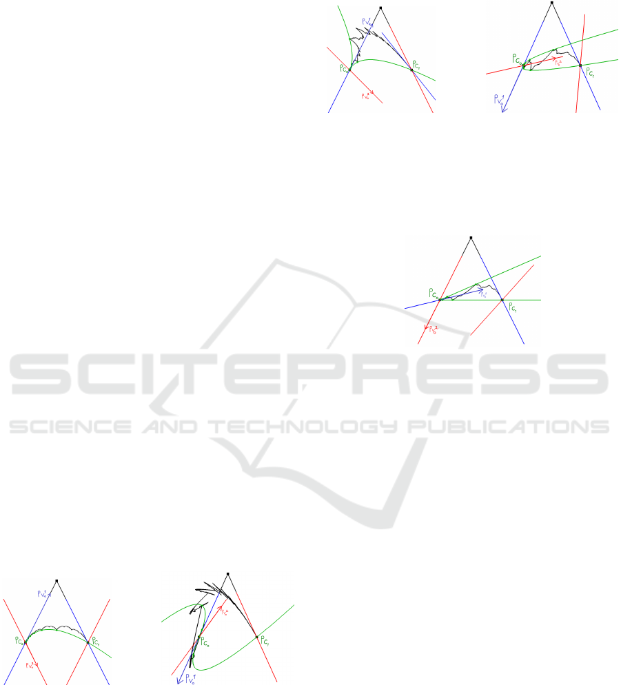
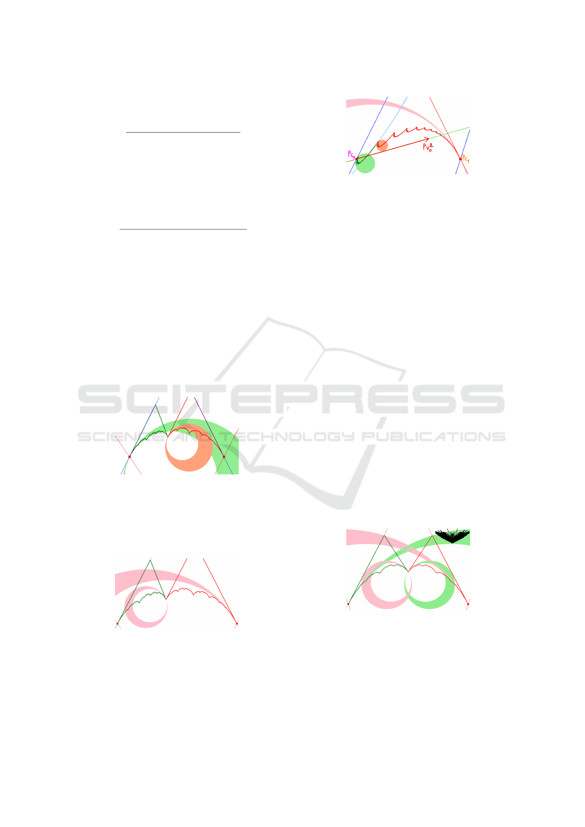
Figure 17 shows in orange the resulting range of os-

culating circles representing the right pseudo-curvature

at the joining point (see Figure 18 for its left pseudo-

curvature). Also, Figure 19 shows the range of osculat-

ing circles at the joining point for the case where λ

< 0

and λ

> 0 (Figure 19).

Figure 17: First, FDCF(0) of the curve in Figure 15 induces

a range of osculating circles (illustrated in green) at the left

endpoint c

, where κ

0,in f

= 1.492, κ

0,sup

= 0.982. Second,

the range of osculating circles for the right pseudo-curvature

at the joining point is illustrated in orange, where 2.008 ≤

κ ≤ 2.932. For this curve: λ

= (λ

)

= 0.3025 (1 > λ

> 0).

Figure 18: In pink, we show the range of the left pseudo-

curvature (of the curve displayed in Figure 15) at c

0.589 ≤ κ ≤ 0.733 and at the joining point = T

: 2.785 ≤

κ ≤ 3.460. For this curve:λ

= (λ

)

= 0.49 (1 > λ

> λ

0).

Figures 20 to 22 show some examples of fractal

curves deﬁned from the same set of control points. For

Figure 19: In green, osculating circles representing the

range of the right curvatures at the left endpoint c

: 5.555 <

κ < +∞, for both sides of Pc

+ tPv

, and κ = 0 on

+ tPv

. In pink, the left range of osculating circles at

the right endpoint c

( 0.478 ≤ κ ≤ 0.525). In orange and

blue, the right and left ranges of osculating circles at the

joining point (9.492 < κ < +∞ and 0.115 ≤ κ ≤ 0.126 re-

spectively). For this curve: λ

= −0.35 and λ

= (λ

)

information, we display their associated osculating cir-

cles, distribution of normals (on the top right corner in

black), and we mention their fractal dimension.

First, we consider the case where α = 2. Figures 20

and 21 show two symmetric curves having different right

and left tangents at the joining point (red and green lines

in the ﬁgures), but since each curve is symmetric, i.e. the

operators have the same eigenvalues and eigenvectors,

then we have equal ranges of the left and right curvatures

(κ

and κ

In the speciﬁc case where T

and T

represent the

de Casteljau matrices, we obtain a B

ezier curve, with

a unique DCF which is the Bernstein polynomial basis

functions.

Secondly, when 1 < α < 2, κ

= κ

= 0, meaning the

osculating circle is a straight line. Figure 22 left shows a

fractal curve for which at, any point, the curve seems to

jump suddenly in the direction of the tangent, which cor-

responds to the osculating “circle” (see the endpoints and

the joining point). Finally, when α > 2, κ

= κ

= +∞,

meaning the osculating circle is reduced to a point. Fig-

ure 22 right shows a fractal curve for which, at any point,

the curve seems to turn sharply in a different direction

from the tangent.

Figure 20: At the joining point, we display the right and left

sets of osculating circles with: 2.375 ≤ κ

= κ

≤ 2.958.

For this curve: the fractal dimension is 1.021. α

i,2

= 2 and

= (λ

)

= 0.36.

From the previous Figures (17 to 22), we can observe

a dependency between the amplitude of the pseudo-

curvature range and the curve’s apparent roughness, as

the values of the fractal dimension show.

Pseudo-Curvature of Fractal Curves for Geometric Control of Roughness

185

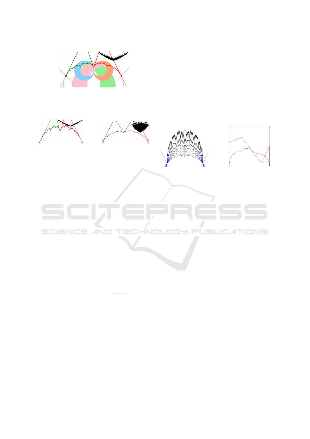
Figure 21: At the joining point, we display the right and left

sets of osculating circles with: 2.808 ≤ κ

= κ

≤ 4.098.

For this curve: the fractal dimension is 1.095, α

i,2

= 2 and

= (λ

)

= 0.4225.

Figure 22: For these two ﬁgures, we focus on the joining

point. Left: α

i,2

= 3 ⇒ κ

= κ

= 0, the fractal dimension

is 1.052, λ

= 0.343 and λ

= 0.7. Right: 1 < α = 1.5 <

2 ⇒ κ

= κ

= +∞, the fractal dimension is 1.007, λ

0.3536, λ

= 0.5, λ

= 0.4079 and λ

= 0.55.

7 DISCUSSION

The DCF has two main interests. First, it highlights the

dynamical behavior of the IFS; we mean how an opera-

tor matches a point of the curve onto another one along

the iteration process, up to the limit ﬁxed point. The

DCF helps to understand and characterize the differen-

tial properties of the curve, as we have shown for the

pseudo-tangent and curvature, which signiﬁcantly im-

pacts the roughness. Second, the DCF is deﬁned from

the IFS operators’ eigensystems. Consequently, we can

ﬁx the eigenvalues and eigenvectors to obtain desired

differential properties. Denoting D the diagonal matrices

of expected eigenvalues and V , the column matrix of the

chosen independent eigenvectors, we can compute the

matrix M of the corresponding operator by M = V DV

−1

The eigenvalue λ

and its associated eigenvector deﬁne

the tangent at the ﬁxed point. Then, we can choose the

value of α by setting λ

= ±λ

(α =

log(|λ

log(λ

)

) to specify

the type of curvature (α < 2 ⇒ κ = ∞, α > 2 ⇒ κ = 0,

α = 2 ⇒ range of curvatures).

Specifying tangents and curvatures at endpoints

(ﬁxed points) is insufﬁcient to control the roughness ac-

curately. The joining point of the two self-similar curve

parts plays a crucial role. Its right and left pseudo-

tangents depend continuously on the endpoints pseudo-

tangents. By adjusting their relative orientations, we can

deﬁne a more or less sharp peak (or valley), which will

be copied along the curve by self-similarity (see Figure

23 left). In (Podkorytov, 2013), Podkorytov shows how

to impose G

(1)

continuity on curves deﬁned by C-IFS.

Using this approach and choosing appropriate eigenval-

ues and eigenvectors, we can deﬁne different left and

right curvatures at the joining point. The resulting curve

is G

(1)

with a speciﬁc ”second-order” roughness (see

Figure 23 right).

In this paper, we give priority to didactic simple ex-

amples. However, complex curves and surfaces can be

produced by increasing the degrees of freedom (d.o.f)

using more than two operators and more control points.

The deterministic self-similarity aspect is not visible

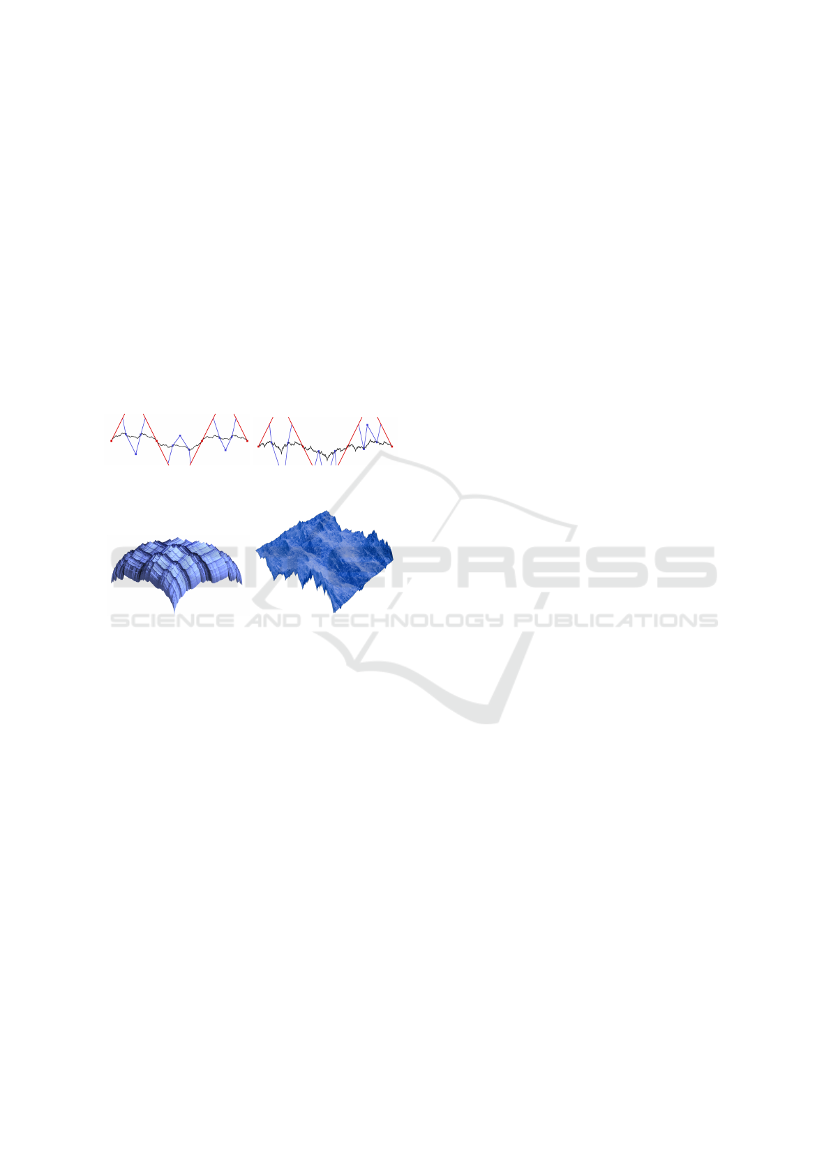
with just a few more d.o.f, producing random-like curves

and surfaces (see Figures 24 and 25 right). Our results

remain for any conﬁgurations, and we have to proceed to

a deep study to understand the relation between pseudo-

curvature and roughness.

Figure 23: Left: a family of curves sharing their sec-

ond eigenvectors (in red) with different orientations of the

pseudo-tangents at endpoints (in blue). The variation of the

valley sharpness, induced by the pseudo-tangent variation,

impacts the roughness. Right: a G

(1)

continuity curve with

a ”second-order” roughness.

8 CONCLUSION

In this study, we propose a method to address the sec-

ond derivative behavior of fractal curves by introduc-

ing a notion of pseudo-curvature. By fractal curves, we

mean self-similar curves described with iterated func-

tion systems (IFS). These curves are completely de-

ﬁned from the set of operators of the IFS and result

from a deterministic iterative process. We introduce the

differential characteristic function (DCF) as a central

tool to analyze the differential behavior of the iterative

computations. We deﬁne a family of DCFs which ab-

stracts the complexity of the iterative process around

each ﬁxed point. Finally, from this family of DCFs,

we obtain a range of curvatures deﬁning the pseudo-

curvature of the fractal curve. We study the different

conﬁgurations of possible pseudo-curvatures according

to operators’ eigenvalues and eigenvectors. These re-

sults, stated for ﬁxed points, are propagated to dyadic

points thanks to the self-similarity property. We pro-

vide examples of various differential situations of frac-

tal curves. The illustrations show, qualitatively, the rel-

evance of this pseudo-curvature, as the range of oscu-

lating circles closely matches the curve. Note that all

results are illustrated with planar fractal curves, but com-

putations are conducted without such an assumption. All

results remain valid for a non co-planar set of control

points deﬁned in R

, inducing a non planar curve. Inde-

pendently of the differential property, the DCF is a use-

GRAPP 2024 - 19th International Conference on Computer Graphics Theory and Applications

186

ful tool to leverage geometric intuition to facilitate the

analysis of self-similar fractals.

These results should be straightforwardly extended

to tensor product surfaces. Their bidirectional structura-

tion generally induces combinations of unidirectional

conﬁgurations. However, we must focus carefully on

non-tensor surfaces, which are more complex construc-

tions that generate surfaces with random appearances

(see Figure 25). For example, complex eigenvalues

avoided for curves will produce interesting vortex effects

for surfaces.

We also have to study the relation between the

roughness and the differentiable characteristics in detail.

Roughness is characterized by oscillation frequency (de-

pending on the operator contraction) and oscillation am-

plitude (depending on the pseudo-tangent and curvature

range). We need to formalize these relations to provide

an intuitive and accurate control of roughness.

Figure 24: Example of two curves designed with 3 opera-

tors and 7 control points.

Figure 25: Left: tensor product surface created from a frac-

tal curves. Right: a more complex non-tensor product frac-

tal surface, built from 4 operators and 8 control points.

REFERENCES

Allaart, P. C. and Kawamura, K. (2010). The improper

inﬁnite derivatives of takagi’s nowhere-differentiable

function. Journal of Mathematical Analysis and Ap-

plications, 372(2):656–665.

Allaart, P. C. and Kawamura, K. (2012). The takagi func-

tion: a survey. Real Analysis Exchange, 37(1):1–54.

Barnsley, M. F. (2014). Fractals everywhere. Academic

press.

Bensoudane, H. (2009). Etude diff

erentielle des formes

fractales. PhD thesis, Universit

e de Bourgogne.

Bensoudane, H., Gentil, C., and Neveu, M. (2009). Frac-

tional half-tangent of a curve described by iterated

function systems. Journal Of Applied Functional

Analysis, 4(2):311–326.

Bigerelle, M., Nianga, J.-M., Najjar, D., Iost, A., Hubert,

C., and Kubiak, K. (2013). Roughness signature of tri-

bological contact calculated by a new method of peaks

curvature radius estimation on fractal surfaces. Tribol-

ogy International, 65:235–247.

Bolzano, B. (1851). Paradoxes of the Inﬁnite. Leipzig, C.H.

Reclam.

Cavalier, A., Gilet, G., and Ghazanfarpour, D. (2019). Lo-

cal spot noise for procedural surface details synthesis.

Computers and Graphics, 85:92–99.

Chermain, X., Sauvage, B., Dischler, J.-M., and Dachs-

bacher, C. (2021). Importance sampling of glittering

BSDFs based on ﬁnite mixture distributions. In Proc.

of Eurographics Symposium on Rendering, pages 45–

53.

Cook, R. L. and DeRose, T. (2005). Wavelet noise. ACM

Trans. Graph., 24(3):803–811.

Daoudi, K., L

evy V

ehel, J., and Meyer, Y. (1998). Con-

struction of continuous functions with prescribed local

regularity. Constructive Approximation, 14:349–385.

Fournier, A., Fussell, D., and Carpenter, L. (1982). Com-

puter rendering of stochastic models. Communica-

tions of the ACM, 25(6):371–384.

Gentil, C., Gouaty, G., and Sokolov, D. (2021). Geometric

Modeling of Fractal Forms for CAD. John Wiley &

Sons.

Gilet, G., Sauvage, B., Vanhoey, K., Dischler, J.-M.,

and Ghazanfarpour, D. (2014). Local random-phase

noise for procedural texturing. ACM Trans. Graph.,

33(6):1–11.

Hardy, G. H. (1916). Weierstrass’s non-differentiable func-

tion. Transactions of the American Mathematical So-

ciety, 17(3):301–325.

Hu, Y. Z. and Tonder, K. (1992). Simulation of 3-D random

rough surface by 2-D digital ﬁlter and fourier analysis.

International Journal of Machine Tools and Manufac-

ture, 32(1-2):83–90.

Hutchinson, J. (1981). Fractals and self-similarity. Indiana

Univ. Math. J., 30:713–747.

Lagae, A., Lefebvre, S., Drettakis, G., and Dutr

e, P. (2009).

Procedural Noise using Sparse Gabor Convolution.

ACM Transactions on Graphics, 28(3):54–64.

Mandelbrot, B. B. (1977). Fractals: Form, Chance, and

Dimension. W.H. Freeman.

Moalic, H., Fitzpatrick, J., and Torrance, A. (1987). The

correlation of the characteristics of rough surfaces

with their friction coefﬁcients. Proc. of the Institution

of Mechanical Engineers, Part C: Journal of Mechan-

ical Engineering Science, 201(5):321–329.

Morlet, L., Gentil, C., Lanquetin, S., Neveu, M., and Baril,

J.-L. (2019). Representation of nurbs surfaces by con-

trolled iterated functions system automata. Computers

& Graphics, 2:100006.

Nayak, S. R., Mishra, J., and Palai, G. (2019). Analysing

roughness of surface through fractal dimension: A re-

view. Image Vis. Comput., 89:21–34.

Nowicki, B. (1985). Multiparameter representation of sur-

face roughness. Wear, 102(3):161–176.

Pavie, N. (2016). Mod

elisation par bruit proc

edural et

rendu de d

etails volumiques de surfaces dans les

enes virtuelles. PhD thesis, Universit

e de Limoges.

Perlin, K. (1985). An image synthesizer. SIGGRAPH Com-

put. Graph., 19(3):287–296.

Pseudo-Curvature of Fractal Curves for Geometric Control of Roughness

187

Podkorytov, S. (2013). Tangent spaces for self-similair

shapes. Phd thesis, Universit

e de Bourgogne.

erez-R

afols, F. and Almqvist, A. (2019). Generating ran-

domly rough surfaces with given height probability

distribution and power spectrum. Tribology Interna-

tional, 131:591–604.

Schaefer, S., Levin, D., and Goldman, R. (2005). Subdivi-

sion Schemes and Attractors. Symposium on Geome-

try Processing, pages 171–180.

Sokolov, D., Gouaty, G., Gentil, C., and Mishkinis, A.

(2015). Boundary controlled iterated function sys-

tems. In Curves and Surfaces: 8th International Con-

ference, Paris, pages 414–432.

Stam, J. (2001). An illumination model for a skin layer

bounded by rough surfaces. In Proc. of the Eurograph-

ics Workshop on Rendering Techniques, page 39–52.

Thim, J. (2003). Continuous Nowhere Differentiable Func-

tions. Master’s thesis, Lule

a University of Technol-

ogy.

Walter, B., Marschner, S. R., Li, H., and Torrance, K. E.

(2007). Microfacet models for refraction through

rough surfaces. In Proc. of the Eurographics Confer-

ence on Rendering Techniques, page 195–206.

Wang, Y., Azam, A., Wilson, M. C., Neville, A., and Mo-

rina, A. (2021). Generating fractal rough surfaces with

the spectral representation method. Proc. of the In-

stitution of Mechanical Engineers, Part J: Journal of

Engineering Tribology, 235(12):2640–2653.

Warszawski, K. K., Nikiel, S. S., and Mrugalski, M. (2019).

Procedural method for fast table mountains modelling

in virtual environments. Applied Sciences, 9(11).

Whitehouse, D. J. (1982). In Rough surfaces (Ed. T. R.

Thomas). Digital techniques.

Zair, C. E. and Tosan, E. (1996). Fractal modeling us-

ing free form techniques. Computer Graphics Forum,

15(3):269–278.

GRAPP 2024 - 19th International Conference on Computer Graphics Theory and Applications

188