Exploring Unsupervised Domain Adaptation Approaches for Water

Parameters Estimation from Satellite Images

Mauren Louise Sguario Coelho de Andrade

, Anderson Paulino Souza

, Bruno Oliveira

Maria Clara Starling

, Camila Costa Amorim

and Jefersson A. dos Santos

Universidade Tecnol

ogica Federal do Paran

a, Ponta Grossa, Paran

a, Brazil

Universidade Federal de Minas Gerais, Belo Horizonte, Minas Gerais, Brazil

Department of Computer Science, University of Shefﬁeld, Shefﬁeld, U.K.

Keywords:

Domain Adaptation, Remote Sensing, Imbalanced Data.

Abstract:

In this paper, we compare several domain adaptation approaches in classifying water quality in reservoirs

using spectral data from satellite images to two optical parameters: turbidity and chlorophyll-a. This assess-

ment adds a new possibility in monitoring these water quality parameters, in addition to the traditional in-situ

investigation, which is expensive and time-consuming. The study acquired images from two data sources

characterized by different geographic regions (USA and Brazil) and veriﬁed the inference quality of the model

trained in the source domain on samples from the target domain. The experiments used two classiﬁers, OS-

CVM and ANN, for domain adaptation methods based on instances, features, and depth. The results suggest

domain adaptation is an efﬁcient alternative when labeled data is scarce. Furthermore, we evaluate the need to

handle imbalanced data, a characteristic of real-world problems like the data explored here. Based on promis-

ing accuracy results, we show that applying domain adaptation techniques in databases with little data, such

as the Brazilian database, and without labeled data, is an efﬁcient and low-cost alternative that can be useful

in monitoring reservoirs in different regions.

1 INTRODUCTION

Big public and private companies are responsible for

building large freshwater reservoirs to meet one or

more human needs, including water supply, ﬂood con-

trol, and power generation. Regardless of its use, wa-

ter quality must be constantly monitored to ensure

safe consumption. However, monitoring water quality

in large reservoirs in situ involves many challenges,

such as high costs, travel across large areas, and dif-

ﬁculty accessing speciﬁc locations. Monitoring water

quality via remote sensing (RM) is a simple alterna-

tive to design and implement at a relatively low cost.

Optical water quality parameters such as turbidity and

chlorophyll can be determined by integrating machine

learning (ML) algorithms and satellite imagery (Zhu

et al., 2022; Li et al., 2022).

However, working with large volumes of labeled

data is one of the biggest challenges. Therefore, the

scientiﬁc community has sought alternatives to the

problem of scarcity of labeled data to enable and ex-

pand the use of techniques in these challenging sit-

uations (Masud, 2012), (Li et al., 2020), (Oza et al.,

2023). One of these techniques is Domain Adaptation

(DA), a concept in ML that refers to the ability to ap-

ply a trained model in a speciﬁc context to a different

context where data distributions may differ. DA can

be employed in classiﬁcation tasks such as classifying

RM images (Tuia et al., 2016), (Zheng et al., 2022).

The scientiﬁc community discusses the evalua-

tion of water quality parameters in satellite images

through ML techniques (Wagle et al., 2020; Krish-

naraj and Honnasiddaiah, 2022; Tian et al., 2023),

employing temporal analysis approaches, parameter

estimation through regression and anomaly detection

methods. Other works investigated the application

of DA in RM and other applications (Elshamli et al.,

2017; Tuia et al., 2021; Luo and Ji, 2022). That said,

a signiﬁcant contribution of this article is a new study

in the area, which applies DA techniques for assessing

water quality in satellite images.

The hypothesis is: if the labeled data from the

image database (USA) have different probability dis-

tributions but with the same characteristics of other

reservoirs in other regions, such as the Tr

es Marias

reservoir, Minas Gerais, Brazil. Is it possible that they

could be used to classify water quality parameters in

such different regions? This work proposes a new

methodology for classifying water quality parameters

to answer this hypothesis. For that, two optical wa-

Coelho de Andrade, M., Souza, A., Oliveira, B., Starling, M., Amorim, C. and Santos, J.

Exploring Unsupervised Domain Adaptation Approaches for Water Parameters Estimation from Satellite Images.

DOI: 10.5220/0012574500003660

Paper published under CC license (CC BY-NC-ND 4.0)

In Proceedings of the 19th International Joint Conference on Computer Vision, Imaging and Computer Graphics Theory and Applications (VISIGRAPP 2024) - Volume 2: VISAPP, pages

861-868

ISBN: 978-989-758-679-8; ISSN: 2184-4321

861

ter quality parameters were chosen for the analysis:

chlorophyll-a (µg/L) and turbidity (NTU), and seven

DA techniques, MDD (Zhang et al., 2019), fMMD

(Uguroglu and Carbonell, 2011), KMM (Huang et al.,

2006), DANN (Ganin et al., 2016), WDGRL (Shen

et al., 2018), CDAN (Long et al., 2018), KLIEP

(Sugiyama et al., 2007) were tested in two classi-

ﬁers: One Class Support Vector Machine (OCSVM)

(Sch

olkopf et al., 1999) and Artiﬁcial Neural Net-

works (ANN) (Mahmon and Ya’acob, 2014).

The main contributions of this paper can be sum-

marized based on three signiﬁcant aspects: (i) We

propose a new methodology to classify water qual-

ity parameters (turbidity and chlorophyll-a) in satel-

lite images, adding DA techniques. The methodol-

ogy uses two different classiﬁers to classify turbid-

ity and chlorophyll-a values, OCSVM and ANN, and

we will compare them to determine the methodo-

logy’s applicability; (ii) The methodology used the

American reservoir database to classify turbidity and

chlorophyll-a values through DA and then apply DA

to classify the Tres Marias data set. Promising ex-

perimental results should motivate the application of

the methodology to different reservoirs regardless of

geographic location; and, (iii) We have employed the

SMOTE method to deal with the problem of imbal-

ance between classes through the comparative anal-

ysis of the accuracy values with and without DA in

both scenarios: using data balanced by the SMOTE

method and unbalanced data.

2 BACKGROUND AND RELATED

WORK

This study used and evaluated different DA tech-

niques to solve the problem of classifying water qual-

ity parameters in reservoirs using RM image data.

This section brieﬂy summarizes the DA notation and

its primary division.

We use D

to denote the source domain and D

denote the target domain. The samples in the set and

their corresponding labeling in D

are given by X

,...,x

} and Y

= {y

,...,y

} with x

∈ R

and

∈ {1, 2, ...,C}, where n

is the number of labeled

samples, D is the dimensionality and C is the number

of classes. In this work, the problem of classifying

turbidity and chlorophyll-a parameters falls under un-

supervised DA, in which there is no labeling in the tar-

get domain. The target domain will have an unlabeled

database X

= {x

,...,x

} where n

is the number of

target samples (Peng et al., 2022).

Since the probability distribution between the

source domain and target domain is different, the la-

Table 1: A brief summary of the existing works on DA

methods for the Classiﬁcation of Remote Sensing Data.

Author Application Method

(Zhang et al., 2022), Road segm. Deep DA

(Ji et al., 2021) Land Cover Class. Deep DA

(Liu and Qin, 2020) Land Cover Class. Feature-based

(Yan et al., 2022) Various Feature-based

(Yan et al., 2018) Scene class. Instance-based

(Liu and Li, 2014) Land Use class. Instance-based

bel space of the source domain and the label space of

the target domain are also different. The idea is to

create a new representation space with the features of

the data that belong to the source class and that, at the

same time, exist in the target class. In this way, a clas-

siﬁer will be trained on the labeled source data so that

it can later be safely applied to the unlabeled target

data. DA methods can be divided into traditional shal-

low methods and, more recently, deep DA methods.

Traditional methods can be based on instances, fea-

tures (both used in this work), and classiﬁers to mini-

mize distances between domains. Deep DA methods

use CNN, autoencoder, or adversarial to reduce the

gap between domains (Wambugu et al., 2021), (Peng

et al., 2022). Table 1 summarizes the works with the

DA methods characterized by traditional and deep DA

methods observed in RM problems.

The instance-based DA methods handle shifts be-

tween data distributions, minimizing target risk using

the source’s labeled data. In this type of adjustment,

only the marginal distributions of the source or tar-

get samples are considered to align the distribution of

the domains. In the feature-based approaches the ba-

sic idea is to transform source and target data into a

feature space, mapping so that the data distribution

is similar. In other words, the method learns a trans-

formation that extracts the representation of invariant

features across domains. Then, the method minimizes

the gap between domains in the new representation

space in an optimization procedure while preserving

the underlying structure of the original data. In this

case, adaptation is performed by the joint extraction

of features, typically based on subspace and transfor-

mation. The deep learning DA adds adaptation layers

to an original deep network architecture to perform

source-target transformation or adopts an adversarial

learning strategy to minimize cross-domain discrep-

ancy (Farahani et al., 2021), (Peng et al., 2022).

3 MATERIALS AND METHODS

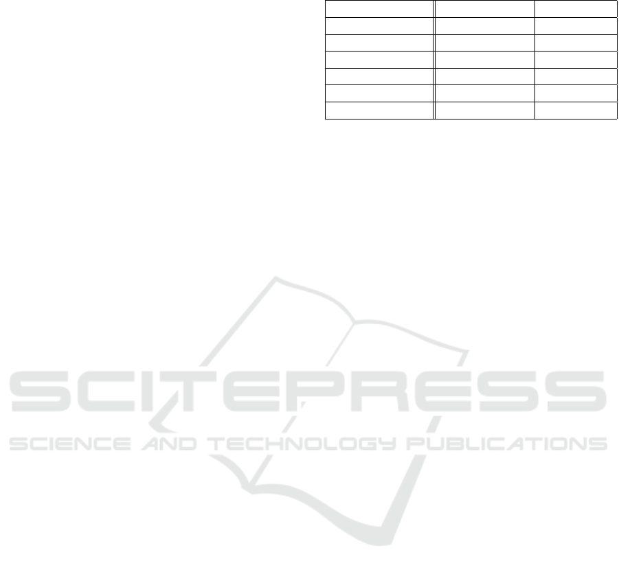
Figure 1 describes the developed methodology. The

basic idea is to assign labels to the data from the struc-

VISAPP 2024 - 19th International Conference on Computer Vision Theory and Applications

862

tured databases (USA and Tr

es Marias) according to

the binary classiﬁcation criteria deﬁned for the turbid-

ity and chlorophyll-a parameters. Using Google Earth

Engine services, this labeled data is merged with the

reﬂectance values of the satellite image pixels (Fig-

ure 1 - 1). Next, the values are ﬁltered to avoid neg-

ative data quality due to spectral noise, clouds, and

shadows (Figure 1 - 2). Then, the database is divided

into the source domain and target domain according

to the criteria established for each experiment (Figure

1 - 3). It is essential to mention that the target domain

does not use labeled data. So, our experiments are

classiﬁed as unsupervised, where the source domain

has labeling data and the target domain does not. An

optional step is added to handle the imbalanced data

issue (Figure 1 - 4). Subsequently, the two classiﬁers,

OCSVM and ANN, are trained without DA and with

the 7 DA methods (Figure 1 - 5). Finally, the result of

each experiment is compared to analyze the applica-

bility of the methodology (Figure 1 - 6).

3.1 Database

The structured database used in this research rep-

resents the dependent variables (which will be pre-

dicted/estimated). The parameters explored were tur-

bidity and chlorophyll-a: (A) In situ campaigns (Tr

Marias, Brazil, shown in Figure 2a). The in situ water

sample collection points are red in Figure 2a. Wa-

ter quality parameters were sampled through in situ

campaigns carried out between 2019 and 2022, in

periods of ﬂood and drought, distributed along the

es Marias Reservoir—sampling objects: physical-

chemical parameters of surface water. (B) United

States of America (illustrated in Figure 2b and 2c) -

The US National Water Quality Monitoring Program

provides a long-term historical basis of physicochem-

ical parameters of water quality

It was necessary to deﬁne standard measurement

units for each evaluated water quality parameter: µg/l

for chlorophyll-a and NTU for turbidity.

3.2 RM Data Acquisition

Spectral data from the Sentinel-2 satellite were used

to develop the methodology. The applied data under-

went atmospheric correction (surface reﬂectance) and

orthorectiﬁcation processes, and the spectral bands

were resampled (when necessary) to a spatial reso-

lution of 20 m. This resolution was deﬁned because

it presented a lower level of interference/noise during

the statistical analysis of the reﬂectance of pixel val-

ues. In order to mitigate harmful data quality aspects

Resource access: https://www.waterqualitydata.us/.

arising from spectral noise, clouds, and shadows, a

combination of ﬁlters, indices, and auxiliary proper-

ties of the satellite image was applied: cloud detection

masks (MSK CLDPRB and QA60); snow/ice masks

(MSK SNWPRB); pixel classiﬁcation, SCL (Scene

Classiﬁcation); Normalized Difference Water Index

(NDWI); Snow Detection Index, Non-Binary Snow

Index for Multi-Component Surfaces (NBSI)

An algorithm in Python, CaptGeo, was developed

to extract the reﬂectance values of pixels from the

spectral bands of satellite images. The algorithm

computes and extracts pixel values from the Google

Earth Engine cloud platform. The application re-

ceives as input data a structured ﬁle with the measure-

ments of a parameter (turbidity, chlorophyll-a) and

their respective geographic coordinates, from which

the location and reﬂectance value of the pixel corres-

pond to each one of the spectral bands available in

the satellite image. After processing, a structured ﬁle

with the turbidity and chlorophyll-a data and the val-

ues of the spectral bands referring to each geographic

coordinate corresponds to the data that will be used as

input in the ML models.

3.3 Experimental Results

Google Colab was used to implement the methodo-

logy, with the Python 3.6 programming language

and the Scikit-learn and Adapt libraries (de Mathe-

lin et al., 2021), (Pedregosa et al., 2011), (Bisong,

2019). The metrics considered to evaluate the results

obtained in adapting the domain were accuracy and

balanced accuracy. The neural network used has two

intermediate layers with ten neurons each. The output

layer is a sigmoid function; it will set class 0 or 1 de-

pending on the threshold. Initially, the US database

was chosen to classify turbidity and chlorophyll-a

values. For this, the database was divided into two

groups: longitudes at 96.9915° W (named here by

ﬁrst division - FD, illustrated in Figure 2b) and the

second latitude at 36.9915° N (named now second di-

vision - SD, showing in Figure 2c). We obtained the

two databases, FD and SD, based on the longitude and

latitude values. In this way, testing two antagonis-

tic scenarios/environments with different biomes was

possible.

Both datasets FD and SD were divided again to

create the source domain and target domain; the two

classiﬁers (OCSVM and ANN) were used for training

the source domain, and the target domain was used

for testing, without using labeling data. The binary

For a detailed explanation of the bands, the number of

pixels, and the ﬁlters used, please consult our previous work

in paper (Souza et al., 2023)

Exploring Unsupervised Domain Adaptation Approaches for Water Parameters Estimation from Satellite Images

863

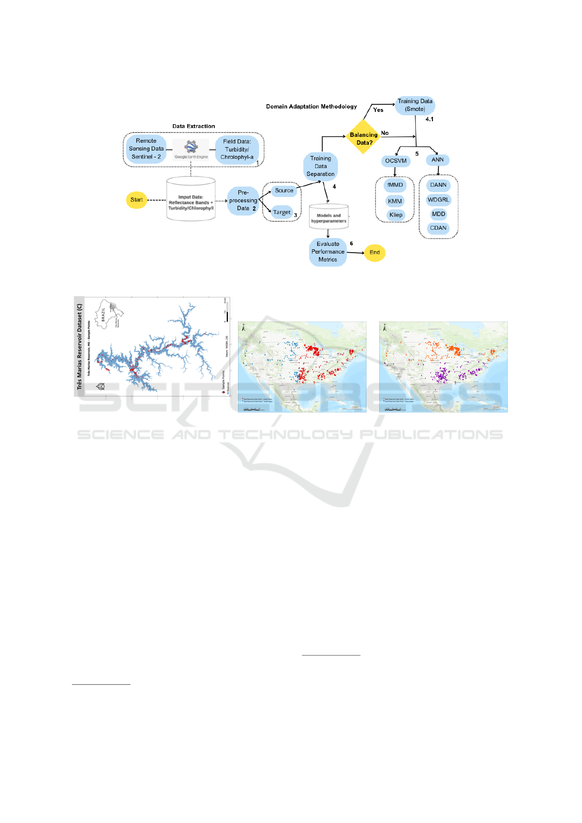
Figure 1: Overview of the proposed Domain Adaptation pipeline.

(a) Map of reservoir data col-

lected from the Tr

es Marias,

Brazil.

(b) USA map of reservoir data

divided by FD.

divided by SD.

Figure 2: Brazil and USA reservoir datasets.

classiﬁcation was divided based on a value deﬁned

from a series of studies related to legal standards es-

tablished within the scope of water resources manage-

ment

. The binary division was established as fol-

lows: i) Turbidity - Class 0, values below 25 and Class

1, values above 25 NTU; ii) Chlorophyll-1 - Class 0,

values below 11.03 and Class 1, values above 11.03

µg/L. In this work, binary classiﬁcation proved to

be more accurate, according to the results discussed

in the following subsection. Furthermore, for thresh-

olds below 25 NTU, the separation of pixels becomes

more complex as the reﬂectance values become in-

creasingly similar; therefore, it was observed that the

band variation is sensitive to multiclass classiﬁcation.

After the results of the experiments observed in

the US database, new experiments were designed for

the Brazilian database. The fundamental question to

be answered is the applicability of DA methods in

classifying water quality parameters in reservoirs with

https://www.epa.gov/dwreginfo/drinking-water-

regulations; https://www.irishstatutebook.ie/eli/2014/si/122/

a labeled database to other reservoirs with little or no

labeled data. The experiments below seek to answer

this question, especially for geographic differences.

3.3.1 United States Subdivision

Table 2 describes the latlong division of the United

States, the sample number of Source and Target Do-

main, and the sample numbers according to the class

division for turbidity and chlorophyll-a values.

Table 3

describes the balanced accuracy values

for 25 NTU (Nephelometric Turbidity Units) and

11.03 µg/L divided by regions according to the men-

tioned above. The ﬁrst classiﬁer tested in this case

was the OCSVM without DA. Then, the same classi-

ﬁer was used to train the database with the three dif-

ferent DA methods (KLIEP, KMM - instance-based,

The red color in the table indicates that the classiﬁca-

tion without DA obtained higher accuracy values than us-

ing DA (negative transfer). The green color indicates that

the classiﬁcation with DA obtained a higher accuracy value

than without DA (positive transfer).

VISAPP 2024 - 19th International Conference on Computer Vision Theory and Applications

864

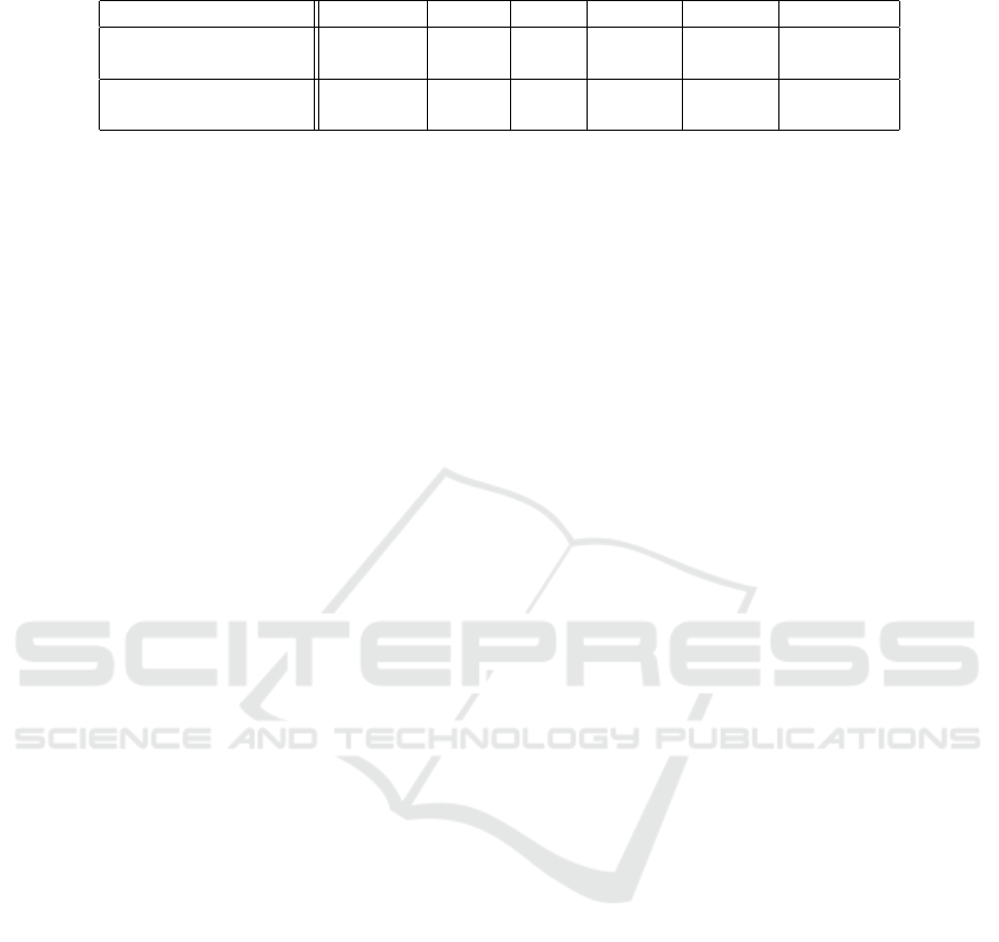
Table 2: United States longitude and latitude divisions - turbidity and chlorophyll-a values.

Parameter Long/Lat Source Target Class 0 Class 1 NTU/µg/L

Turbidity FD 1637 225 1533 104 25

Turbidity SD 1347 515 1243 104 25

Chlorophyll-a FD 4029 465 2517 1512 11.03

Chlorophyll-a SD 2186 2308 1277 909 11.03

and fMMD - feature-based). The balanced accuracy

values described in Table 3 show that DA improved

accuracy for all experiments. We can observe that the

Kmm, and fMMD methods stand out when classify-

ing the turbidity parameter. The Kernel Mean Match-

ing - KMM method is an instance-based sample bias

correction that minimizes the maximum mean dis-

crepancy (MMD) between the source and target do-

mains. The algorithm corrects for the difference be-

tween the input source and target distributions by pre-

weighting the source instances to minimize the differ-

ence between the training/test point means in a Repro-

duction Kernel Hilbert Space (RKHS) (Huang et al.,

2006). The fMMD method is feature-based, using in-

put features to minimize the maximum mean discrep-

ancy (MMD) between the source and target data.

Table 3 also describes the classiﬁcation by RNA

without DA and by RNA and four DA methods

(DANN, WDGRL, MDD, and CDAN). The high-

light of these experiments was the WDGRL method

that works on adversarial neural network architec-

tures. The discriminator approximates the Wasser-

stein distance between the encoded source and target

distributions based on WGAN (Wasserstein Adver-

sarial Generative Network) (Arjovsky et al., 2017).

For the chlorophyll-a results (Table 3 on the right),

we can highlight the values obtained by KMM with

OCSVM, DANN, and CDAN with ANN. The DANN

method aims to ﬁnd a new representation of the in-

put features in which any discriminator network can-

not distinguish the source and target data. This new

representation is learned by a network of encoders

in an adversarial manner. A task network is learned

in the coded space parallel to the encoder and dis-

criminator networks. In the CDAN method, the dis-

criminator is conditioned on the prediction of the task

network for source and target data. Thus, the focus

is on the source-destination correspondence between

instances belonging to the same (de Mathelin et al.,

2021) class. For both OSCVM and ANN, the results

suggest that applying DA to classify the chlorophyll

parameter is more appropriate, thus ensuring a better

response from the classiﬁer with unbalanced data and

without labeling in the target domain.

The table 4 describes the balanced precision val-

ues per class using the Synthetic Minority Over-

sampling (SMOTE) technique (Chawla et al., 2002).

Smote synthesizes new samples based on existing

samples; therefore, the new data generated, closer to

the real data, promotes balance in the class. The ac-

curacy values described in Table 4 show that apply-

ing DA has the highest accuracy compared to classi-

ﬁcation without DA. Only in two scenarios using the

ANN classiﬁer can we observe the presence of neg-

ative transfer for turbidity and chlorophyll-a. Nega-

tive transfer occurs when the application of DA tech-

niques impairs classiﬁer performance. Still, it is pos-

sible to highlight the accuracy values of the TrAd-

aBoost, KMM, and KLIEP methods in the classiﬁca-

tion by OSCVM DANN and CDAN again for ANN.

The KLIEP method, also an instance-based method,

corrects for the difference between the input distri-

butions of the source and target domains through a

reweighting of the source instances that minimizes the

Kullback-Leibler divergence between the source and

target distributions (Wen et al., 2015).

So far, results indicate an advantage when apply-

ing DA to both classiﬁers to classify turbidity and

chlorophyll-a values in reservoirs, surpassing the ac-

curacy value without DA in most experiments. How-

ever, for balanced data by Smote, deep-based methods

obtained negative transfer in two scenarios. For the

rest of the experiments, it was possible to observe that

the KMM and fMMD method got promising results in

most OSCVM experiments, followed by DANN and

CDAN by ANN.

3.3.2 Tr

es Marias Reservoir

The following experiments used the complete US

database as the source domain (without dividing it by

longitude and latitude) and, database from the Tr

Marias reservoir, Minas Gerais, Brazil, was used as

the target domain. An illustration of chlorophyll-a

data in 2 dimensions is shown in Figure 3a before the

DA method application. Source data is shown in blue

(USA), and target data is shown in red (Tr

es Marias).

Figure 3b illustrates the distribution of features after

applying the instance-based method. Figure 3c af-

ter applying the feature-based method and Figure 3d

after applying the deep-based DA method. Interest-

ingly, the distribution resulting from the deep method

is similar to that from the feature-based. This is be-

cause deep-base methods also use strategies that in-

Exploring Unsupervised Domain Adaptation Approaches for Water Parameters Estimation from Satellite Images

865

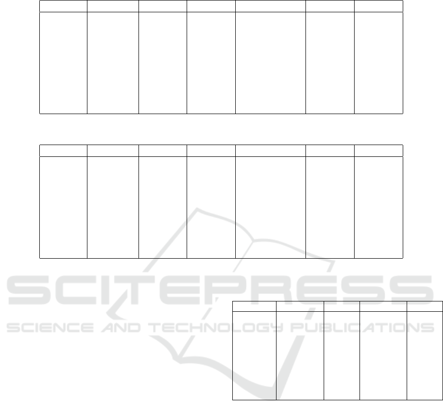
Table 3: Turbidity and Chlorophyll-a - USA division - Unbalanced Data - Balanced Accuracy.

Method Parameter FD SD Parameter FD SD

OCSVM

Turbidity

0.695206 0.637180

Chlorophyll-a

0.770352 0.713083

Kliep 0.676338 0.657131 0.762072 0.719558

KMM 0.752523 0.656824 0.788668 0.709516

fMMD 0.704640 0.711570 0.752960 0.695959

ANN 0.717694 0.702136 0.792831 0.809472

DANN 0.676338 0.718839 0.812211 0.830679

WDGRL 0.771391 0.715593 0.812165 0.807481

MDD 0.661090 0.657131 0.774838 0.823180

CDAN 0.654563 0.697807 0.803469 0.837994

Table 4: Turbidity and Chlorophyll-a - USA division - Balanced Data by SMOTE - Accuracy.

Method Parameter FD SD Parameter FD SD

OCSVM

Turbidity

0.831111 0.895146

Chlorophyll-a

0.752688 0.729203

Kliep 0.848889 0.916505 0.726882 0.709272

KMM 0.871111 0.904854 0.765591 0.790295

fMMD 0.822222 0.897087 0.769892 0.744367

ANN 0.826667 0.842718 0.817204 0.830589

DANN 0.848889 0.834951 0.804301 0.816724

WDGRL 0.813333 0.831068 0.800000 0.810225

MDD 0.831111 0.833010 0.804301 0.818891

CDAN 0.844444 0.819417 0.808602 0.832322

vestigate standard features with similar behavior con-

cerning the task in the source and target domains.

Then, generating a new feature representation to cor-

rect the difference between the source and target dis-

tributions. In Figure 3b, however, based on instances,

it is possible to notice the attempt to reweight the data

to correct the difference between the source and target

distributions.

Table 5 describes the balanced accuracy values

for Turbidity classiﬁcation using the US source and

es Marias target domains. We can observe in Table

5 the good results of the balanced accuracy, mainly

considering the KMM and fMMD methods. This

result was expected, as these method have already

shown promising results in the previous experiments,

as mentioned earlier. These values prove the advan-

tage of using DA to classify turbidity in different

reservoirs, even in distant geographical positions.

Table 5 also describes the balanced precision val-

ues for the classiﬁcation of chlorophyll-a considering

the limit of 11.03 µg/L. This limit value was cho-

sen based on the literature information described pre-

viously. The accuracy values of the KMM, fMMD,

and WDRGL methods suggest that using DA for the

es Marias database with little data available is better

than without DA. We also improved the classiﬁer’s re-

sponse for the classiﬁcation of chlorophyll-a. There-

fore, by analyzing all the experiments carried out, it

is possible to answer the question of the applicabil-

Table 5: Turbidity (T) and Chlorophyll-a (C) - Tr

es Maria’s

Target - Balanced Accuracy.

Method Parameter 25 Parameter 11.03

OCSVM T 0.7312 C 0.5963

KLIEP T 0.5588 C 0.5342

KMM T 0.7325 C 0.6310

fMMD T 0.7620 C 0.6234

ANN T 0.8208 C 0.7515

DANN T 0.8488 C 0.6932

WDGRL T 0.8194 C 0.7581

MDD T 0.6149 C 0.7378

CDAN T 0.8181 C 0.6960

ity of DA in data from labeled global reservoirs to

other reservoirs without labels. In particular, we can

consider the results obtained using AD in databases

with little data promising. This is the case with the

es Marias database, which has scarce labeling data

attesting to the model’s applicability. A simple al-

gorithm can be implemented and made available to

Brazilian reservoir managers. The idea is to create an

algorithm to classify turbidity and chlorophyll-a val-

ues, automatically choosing the one with the highest

accuracy values. This ensures that the algorithm al-

ways selects the method with the highest accuracy

values for each classiﬁcation, whether turbidity or

chlorophyll-a.

VISAPP 2024 - 19th International Conference on Computer Vision Theory and Applications

866

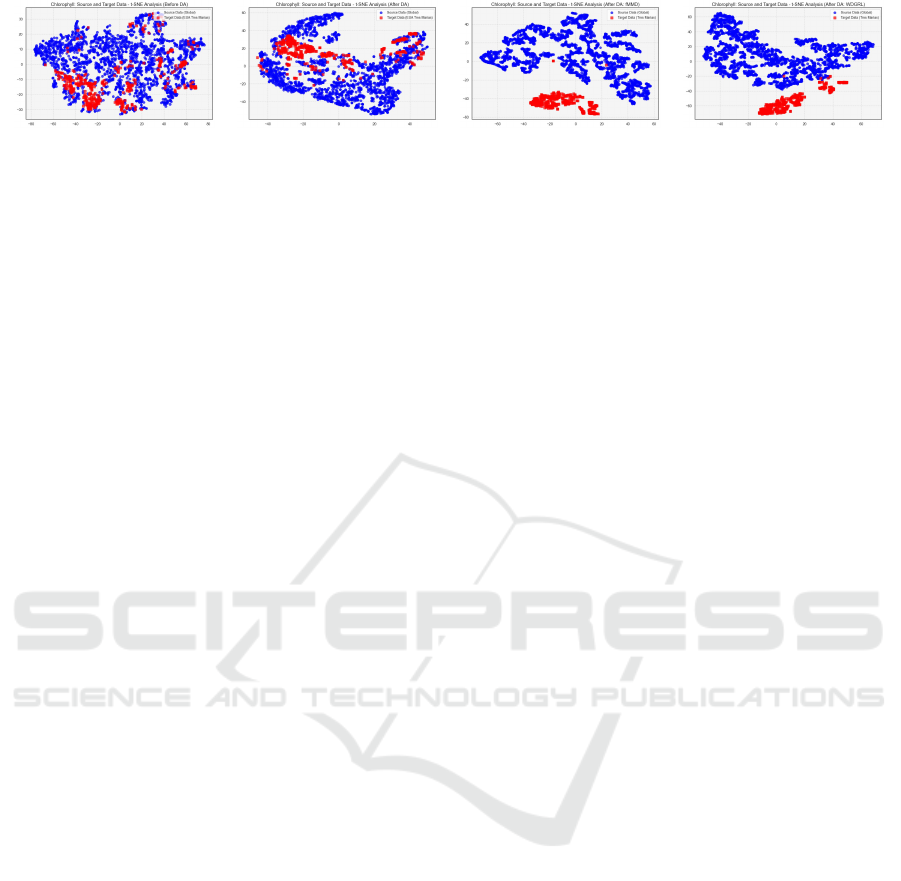
(a) Before DA. (b) Instance based. (c) Feature based. (d) Deep based.

Figure 3: Chlorophyll-a data distribution by t-SNE Analysis.

4 CONCLUSION

This study presented the performance of seven do-

main adaptation techniques (Kliep, KMM, fMMD,

DANN, WDGRL, MDD, and CDAN) in classifying

water quality in reservoirs using spectral data from

satellite images to two optical parameters: turbidity

and chlorophyll-a. We used the US database as the

target domain to classify turbidity and chlorophyll

values from the Tr

es Marias database, which has lit-

tle and unlabeled data. The hypothesis analyzed was

whether labeled data from the image database (USA)

with different probability distributions but with the

same characteristics from other reservoirs in other re-

gions (Brazil) could be used to classify water quality

parameters in reservoirs using DA. To this end, we

use two classiﬁers, OSCVM and ANN, and data aug-

mentation by the SMOTE method to solve the class

imbalance problem.

We observed that in most of the DA techniques

tested, the individual performance of each one was

good enough in at least one scenario. Trad-aBoost,

KMM, and fMMD show promising and regular re-

sults for most experiments using the OCSVM classi-

ﬁer. They were followed by CDAN, DAN, and WD-

GRL using the RNA classiﬁer. However, the RNA

classiﬁer presents the problem of negative transfer in

some cases. Still, our experimental results indicate

that using DA to classify turbidity and chlorophyll-a

parameters in reservoirs is a promising solution. With

this, we show that using large trained databases to

classify databases with unlabeled and sparse data with

the help of DA is possible. Monitoring water qual-

ity in large reservoirs could beneﬁt from using remote

sensing images as an efﬁcient and low-cost alternative

that will contribute to in situ monitoring in regions

with little data or difﬁculty obtaining.

ACKNOWLEDGMENTS

The authors gratefully acknowledge the support pro-

vided by Companhia Energ

etica de Minas Gerais

(CEMIG) and Universidade Federal de Minas Gerais

(UFMG) for the development of this work through

project GT-0607: “Intelligent Water Quality Monitor-

ing through the Development of Photo-optical Algo-

rithm”.

REFERENCES

Arjovsky, M., Chintala, S., and Bottou, L. (2017). Wasser-

stein generative adversarial networks. In ICML, pages

214–223.

Bisong, E. (2019). Google colaboratory. In Building Ma-

chine Learning and Deep Learning Models on Google

Cloud Platform, pages 59–64. Springer.

Chawla, N. V., Bowyer, K. W., Hall, L. O., and Kegelmeyer,

W. P. (2002). SMOTE: Synthetic minority over-

sampling technique. Journal of Artiﬁcial Intelligence

Research, 16:321–357.

de Mathelin, A., Deheeger, F., Richard, G., Mougeot,

M., and Vayatis, N. (2021). Adapt: Awesome do-

main adaptation python toolbox. arXiv preprint

arXiv:2107.03049.

Elshamli, A., Taylor, G. W., Berg, A., and Areibi, S. (2017).

Domain adaptation using representation learning for

the classiﬁcation of remote sensing images. JSTARS,

10(9):4198–4209.

Farahani, A., Voghoei, S., Rasheed, K., and Arabnia, H. R.

(2021). A brief review of domain adaptation. Ad-

vances in Data Science and Information Engineering:

Proceedings from ICDATA 2020 and IKE 2020, pages

877–894.

Ganin, Y., Ustinova, E., Ajakan, H., Germain, P.,

Larochelle, H., Laviolette, F., Marchand, M., and

Lempitsky, V. (2016). Domain-adversarial training of

neural networks. The journal of machine learning re-

search, 17(1):2096–2030.

Huang, J., Gretton, A., Borgwardt, K., Sch

olkopf, B., and

Smola, A. (2006). Correcting sample selection bias by

unlabeled data. Neurips, 19.

Ji, S., Wang, D., and Luo, M. (2021). Generative adver-

sarial network-based full-space domain adaptation for

land cover classiﬁcation from multiple-source remote

sensing images. TGRS, 59(5):3816–3828.

Krishnaraj, A. and Honnasiddaiah, R. (2022). Remote sens-

ing and machine learning based framework for the as-

sessment of spatio-temporal water quality in the mid-

Exploring Unsupervised Domain Adaptation Approaches for Water Parameters Estimation from Satellite Images

867

dle ganga basin. Environmental Science and Pollution

Research, 29(43):64939–64958.

Li, R., Jiao, Q., Cao, W., Wong, H.-S., and Wu, S. (2020).

Model adaptation: Unsupervised domain adaptation

without source data. In CVPR, pages 9641–9650.

Li, Y., Dang, B., Zhang, Y., and Du, Z. (2022). Wa-

ter body classiﬁcation from high-resolution optical re-

mote sensing imagery: Achievements and perspec-

tives. ISPRS Journal of Photogrammetry and Remote

Sensing, 187:306–327.

Liu, W. and Qin, R. (2020). A multikernel domain adap-

tation method for unsupervised transfer learning on

cross-source and cross-region remote sensing data

classiﬁcation. TGRS, 58(6):4279–4289.

Liu, Y. and Li, X. (2014). Domain adaptation for land use

classiﬁcation: A spatio-temporal knowledge reusing

method. ISPRS Journal of Photogrammetry and Re-

mote Sensing, 98:133–144.

Long, M., Cao, Z., Wang, J., and Jordan, M. I. (2018). Con-

ditional adversarial domain adaptation. Neurips, 31.

Luo, M. and Ji, S. (2022). Cross-spatiotemporal land-

cover classiﬁcation from vhr remote sensing images

with deep learning based domain adaptation. IS-

PRS Journal of Photogrammetry and Remote Sensing,

191:105–128.

Mahmon, N. A. and Ya’acob, N. (2014). A review on clas-

siﬁcation of satellite image using artiﬁcial neural net-

work (ann). In 2014 IEEE 5th Control and system

graduate research colloquium, pages 153–157. IEEE.

Masud, M.M., W. C. G. J. e. a. (2012). Facing the real-

ity of data stream classiﬁcation: coping with scarcity

of labeled data. Knowledge and Information Systems,

33:213–244.

Oza, P., Sindagi, V. A., Sharmini, V. V., and Patel, V. M.

(2023). Unsupervised domain adaptation of object de-

tectors: A survey. TPAMI.

Pedregosa, F., Varoquaux, G., Gramfort, A., Michel, V.,

Thirion, B., Grisel, O., Blondel, M., Prettenhofer, P.,

Weiss, R., Dubourg, V., et al. (2011). Scikit-learn:

Machine learning in python. the Journal of machine

Learning research, 12:2825–2830.

Peng, J., Huang, Y., Sun, W., Chen, N., Ning, Y., and Du, Q.

(2022). Domain adaptation in remote sensing image

classiﬁcation: A survey. JSTARS, 15:9842–9859.

Sch

olkopf, B., Williamson, R. C., Smola, A., Shawe-Taylor,

J., and Platt, J. (1999). Support vector method for

novelty detection. Neurips, 12.

Shen, J., Qu, Y., Zhang, W., and Yu, Y. (2018). Wasser-

stein distance guided representation learning for do-

main adaptation. In Proceedings of the AAAI Confer-

ence on Artiﬁcial Intelligence, volume 32.

Souza, A. P., Oliveira, B. A., Andrade, M. L., Starling, M.

C. V., Pereira, A. H., Maillard, P., Nogueira, K., dos

Santos, J. A., and Amorim, C. C. (2023). Integrating

remote sensing and machine learning to detect turbid-

ity anomalies in hydroelectric reservoirs. Science of

The Total Environment, 902:165964.

Sugiyama, M., Nakajima, S., Kashima, H., Buenau, P., and

Kawanabe, M. (2007). Direct importance estimation

with model selection and its application to covariate

shift adaptation. In Platt, J., Koller, D., Singer, Y.,

and Roweis, S., editors, Neurips, volume 20. Curran

Associates, Inc.

Tian, S., Guo, H., Xu, W., Zhu, X., Wang, B., Zeng,

Q., Mai, Y., and Huang, J. J. (2023). Remote sens-

ing retrieval of inland water quality parameters us-

ing sentinel-2 and multiple machine learning algo-

rithms. Environmental Science and Pollution Re-

search, 30(7):18617–18630.

Tuia, D., Persello, C., and Bruzzone, L. (2016). Do-

main adaptation for the classiﬁcation of remote sens-

ing data: An overview of recent advances. IEEE Geo-

science and Remote Sensing Magazine, 4(2):41–57.

Tuia, D., Persello, C., and Bruzzone, L. (2021). Re-

cent advances in domain adaptation for the clas-

siﬁcation of remote sensing data. arXiv preprint

arXiv:2104.07778.

Uguroglu, S. and Carbonell, J. (2011). Feature selection

for transfer learning. In Joint European Conference

on Machine Learning and Knowledge Discovery in

Databases, pages 430–442. Springer.

Wagle, N., Acharya, T. D., and Lee, D. H. (2020). Compre-

hensive review on application of machine learning al-

gorithms for water quality parameter estimation using

remote sensing data. Sens. Mater, 32(11):3879–3892.

Wambugu, N., Chen, Y., Xiao, Z., Tan, K., Wei, M., Liu,

X., and Li, J. (2021). Hyperspectral image classiﬁ-

cation on insufﬁcient-sample and feature learning us-

ing deep neural networks: A review. International

Journal of Applied Earth Observation and Geoinfor-

mation, 105:102603.

Wen, J., Greiner, R., and Schuurmans, D. (2015). Cor-

recting covariate shift with the frank-wolfe algorithm.

In Proceedings of the 24th International Conference

on Artiﬁcial Intelligence, IJCAI’15, page 1010–1016.

AAAI Press.

Yan, L., Zhu, R., Liu, Y., and Mo, N. (2018). Tradaboost

based on improved particle swarm optimization for

cross-domain scene classiﬁcation with limited sam-

ples. JSTARS, 11(9):3235–3251.

Yan, Y., Wu, H., Ye, Y., Bi, C., Lu, M., Liu, D., Wu, Q., and

Ng, M. K. (2022). Transferable feature selection for

unsupervised domain adaptation. IEEE Transactions

on Knowledge and Data Engineering, 34(11):5536–

5551.

Zhang, L., Lan, M., Zhang, J., and Tao, D. (2022). Stage-

wise unsupervised domain adaptation with adversarial

self-training for road segmentation of remote-sensing

images. TGRS, 60:1–13.

Zhang, Y., Liu, T., Long, M., and Jordan, M. (2019). Bridg-

ing theory and algorithm for domain adaptation. In In-

ternational Conference on Machine Learning, pages

7404–7413. PMLR.

Zheng, Z., Zhong, Y., Su, Y., and Ma, A. (2022). Do-

main adaptation via a task-speciﬁc classiﬁer frame-

work for remote sensing cross-scene classiﬁcation.

TGRS, 60:1–13.

Zhu, M., Wang, J., Yang, X., Zhang, Y., Zhang, L., Ren, H.,

Wu, B., and Ye, L. (2022). A review of the application

of machine learning in water quality evaluation. Eco-

Environment & Health, 1(2):107–116.

VISAPP 2024 - 19th International Conference on Computer Vision Theory and Applications

868