Vehicle Pose Estimation: Exploring Angular Representations

Ivan Orlov

1,2 a

, Marco Buzzelli

1 b

and Raimondo Schettini

1 c

Department of Informatics, Systems and Communication, University of Milano-Bicocca, Italy

Aramis Group, France

Keywords:

Vehicle Pose Recognition, Viewpoint Estimation, Car Azimuth Estimation, PASCAL3D+,

Angular Regression.

Abstract:

This paper addresses the challenge of azimuth estimation in the context of car pose estimation. Our re-

search utilizes the PASCAL3D+ dataset, which offers a diverse range of object categories, including cars,

with annotated azimuth estimations for each photograph. We introduce two architectures that approach az-

imuth estimation as a regression problem, each employing a deep convolutional neural network (DCNN)

backbone but diverging in their output deﬁnition strategies. The ﬁrst architecture employs a sin-cos represen-

tation of the car’s azimuth, while the second utilizes two directional discriminators, distinguishing between

front/rear and left/right views of the vehicle. Our comparative analysis reveals that both architectures demon-

strate near-identical performance levels on the PASCAL3D+ validation set, achieving a median error of 3.5

◦

which is a signiﬁcant advancement in the state of the art. The minimal performance disparity between the

two methods highlights their individual strengths while also underscoring the similarity in their practical ef-

ﬁcacy. This study not only proposes effective solutions for accurate azimuth estimation but also contributes

to the broader understanding of pose estimation challenges in automotive contexts. The code is available at

https://github.com/ vani-or/car pose estimation.

1 INTRODUCTION

Pose detection revolves around the process of deter-

mining the position and orientation of speciﬁc parts

or features of an object or entity in images or videos.

Historically, the primary motivation for developing

pose detection algorithms was to detect and analyze

human body parts and their relative positions. Over

time, these methodologies have evolved and have

been adapted to cater to various objects, including

cars, enabling applications in ﬁelds as varied as an-

imation, augmented reality, sports analytics, and ve-

hicle damage assessment.

Early techniques employed to estimate pose made

use of part-based models, where individual parts of an

entity (like limbs in humans) were detected and then

assembled to deduce the overall pose (Felzenszwalb

and Huttenlocher, 2005).

Feature-based methods like Scale-Invariant Fea-

ture Transform (SIFT) (David, 2004) marked a sig-

niﬁcant advancement in the ﬁeld, moving beyond ba-

https://orcid.org/0000-0001-9600-8696

https://orcid.org/0000-0003-1138-3345

https://orcid.org/0000-0001-7461-1451

∗

Corresponding author

sic image processing techniques. In this era, geomet-

ric problems like the Perspective-n-Point (PnP) were

critical, where the objective was to deduce an object’s

pose from 2D-to-3D point correspondences (Lepetit

et al., 2009).

The rise of deep learning, and particularly CNNs,

brought a paradigm shift in pose detection methodolo-

gies. Unlike traditional methods, where features had

to be meticulously crafted, CNNs allowed for auto-

matic feature learning from data. Deep learning mod-

els, such as PoseNet (Kendall et al., 2015) and Mask

R-CNN (He et al., 2017), are representative examples

that have showcased the potential of CNNs in pose

estimation tasks.

This paper focuses on improving azimuth estima-

tion in car pose detection. Using the PASCAL3D+

dataset, it presents two architectures based on deep

convolutional neural networks, differing in their treat-

ment of azimuth: one uses a sin-cos representa-

tion, and the other employs directional discrimina-

tors. Both demonstrate advanced performance in pose

estimation. The paper is structured to ﬁrst provide

background, followed by a problem deﬁnition, de-

tailed methodology, evaluation of results, and con-

cludes with discussions and future work.

Orlov, I., Buzzelli, M. and Schettini, R.

Vehicle Pose Estimation: Exploring Angular Representations.

DOI: 10.5220/0012574300003660

Paper published under CC license (CC BY-NC-ND 4.0)

In Proceedings of the 19th International Joint Conference on Computer Vision, Imaging and Computer Graphics Theory and Applications (VISIGRAPP 2024) - Volume 2: VISAPP, pages

853-860

ISBN: 978-989-758-679-8; ISSN: 2184-4321

853

2 RELATED WORKS

Deep learning, particularly CNNs, has signiﬁcantly

advanced car pose estimation. Models like those in

(Mousavian et al., 2017) accurately predict 3D car

bounding boxes from 2D images. (Prokudin et al.,

2018) introduced a probabilistic model for angular

regression, enhancing accuracy and handling varying

image qualities. MonoGRNet (Qin et al., 2019) pro-

vides a uniﬁed approach for 3D vehicle detection and

pose estimation using monocular RGB images, while

(Xiao et al., 2019) developed a generic, ﬂexible deep

pose estimation method.

Addressing training data scarcity and feature ex-

traction, (Su et al., 2015) combined image synthe-

sis and CNNs, and (Grabner et al., 2018) focused

on 3D pose estimation and model retrieval. Innova-

tive techniques like the characteristic view selection

model (CVSM) by (Nie et al., 2020) and a CNN-

based monocular orientation estimation integrating

Riemannian geometry by (Mahendran et al., 2018)

have been proposed.

Car pose estimation is vital in autonomous driv-

ing and insurance sectors, essential for understanding

vehicle orientation and assessing damages. It’s also

crucial in scenarios lacking direct sensor data, where

visual cues are pivotal (Geiger et al., 2012).

2.0.1 The PASCAL3D+ Dataset

Selecting an apt dataset is pivotal in guiding the re-

search process and ensuring the derived outcomes are

reﬂective of the research objectives. Previous work

(Buzzelli and Segantin, 2021) highlighted the impor-

tance of training data that faithfully model the ap-

plication scenario, speciﬁcally for the case of vehi-

cle analysis. For our investigation into car pose es-

timation, with a particular focus on azimuth estima-

tion, the PASCAL3D+ (Xiang et al., 2014) dataset

emerged as a front-runner. A driving factor behind

this choice was the detailed annotations the dataset

offers for each image, notably the azimuth values.

Azimuth estimation, a critical facet of pose detec-

tion, provides insights into an object’s orientation

within a 3D space, as detailed later on in section 3.

PASCAL3D+ alleviates the complexities of deriving

these angles by offering direct data for azimuth esti-

mation, ensuring a more precise and streamlined re-

search methodology.

The PASCAL3D+ dataset, an extension of the

PASCAL VOC dataset, augments the original im-

ages with intricate 3D annotations, laying the foun-

dation for 3D object detection and pose estimation

tasks. A prominent feature of this dataset is its com-

pilation of 5,475 car images, sourced directly from

ImageNet, presenting a myriad of scenarios for re-

searchers to explore. Each car in this dataset is metic-

ulously annotated with a corresponding 3D CAD

model, which enables researchers to juxtapose pose

estimations against a standardized 3D reference. For

cars, the annotations delve deep, offering viewpoints,

bounding boxes, and crucially, azimuth angles.

Several nuances make PASCAL3D+ a challeng-

ing yet rewarding dataset. The presence of occluded

objects simulates real-world complications that algo-

rithms need to account for. Furthermore, the dataset

showcases a wide variance in car makes and models,

capturing the diversity of the automotive world. How-

ever, it is essential to note that while the dataset offers

this diversity, it does not explicitly label the speciﬁc

makes or models.

3 DEFINING AND VISUALIZING

AZIMUTH

In the domain of vehicle pose detection, one of the

paramount tasks is the precise estimation of the vehi-

cle’s orientation in a given image or frame. The key

orientation parameter being focused upon in this re-

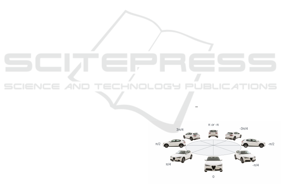
search task is the azimuth, often denoted as ϕ.

The azimuth, ϕ, is deﬁned as the angle in the

range [−π,π] that represents the orientation of a ve-

hicle with respect to the viewer. Originating from the

front of the car, this angle describes how much the ve-

hicle has rotated from this frontal viewpoint. For in-

stance, ϕ = 0 would indicate a car directly facing the

viewer, while ϕ =

would signify the car turned 90

◦

to the right. This deﬁnition is depicted in Figure 1.

Figure 1: Azimuth ϕ deﬁnition for car pose estimation. In

this image, an azimuth of ϕ = −π/4 corresponds to the car

slightly turned to present its right side (passenger side) to-

wards the viewer. Angle 0 represents the reference axis for

this calculation.

It is noteworthy to mention the deliberate exclu-

sion of other viewpoint characteristics from this study,

such as elevation, distance, and the roll equivalent

from roll pitch and yaw. While these parameters can

offer further granularity to pose detection, the primary

VISAPP 2024 - 19th International Conference on Computer Vision Theory and Applications

854

focus here remains the continuous estimation of az-

imuth. When distilled to its essence, the problem

tackled in this research is one of regression. Instead of

the conventional classiﬁcation-based approach where

discrete classes represent different poses or orienta-

tions, the goal here is continuous azimuth estimation.

This involves predicting a speciﬁc value of ϕ for a

given vehicle image. The advantage of this method is

that it allows for a much ﬁner granularity of orienta-

tion prediction.

4 PROPOSED APPROACH

Vehicle pose estimation, especially focusing on the

azimuthal angle, is a multifaceted challenge. While

most regression tasks in deep learning provide con-

tinuous values within a predictable range, the angu-

lar nature of azimuth presents cyclic constraints that

require special consideration. Traditional regression

models would in fact treat angles such as ϕ = π and

ϕ = −π as distinct, ignoring their equality due to the

cyclic nature of angles.

In the context of this research, two distinct

methodologies have been adopted. The common ar-

chitecure is presented in Figure 2, with two different

heads corresponding to the two distinct methodolo-

gies, described in the following.

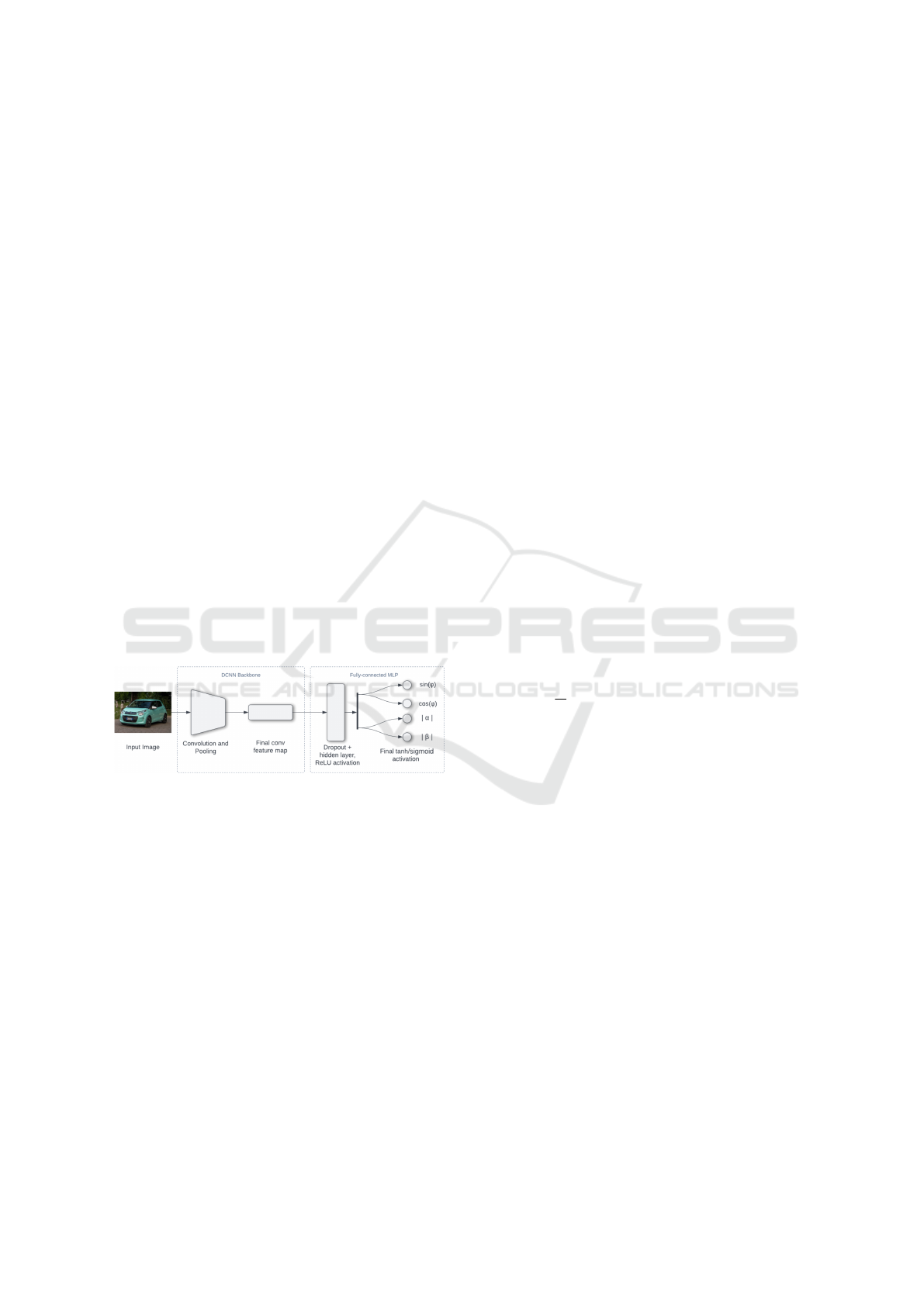
Figure 2: Proposed architecture, with Sin-Cos output repre-

sentation (top head) and Directional Discriminators output

representation (bottom head).

4.1 Sin-Cos Representation

One of the pivotal tasks in vehicle pose estimation

is to represent the azimuthal angle, ϕ, in a format

that can be effectively estimated using deep convolu-

tional neural networks (DCNNs). In addressing this,

our ﬁrst proposed architecture adopts what is referred

to in (Beyer et al., 2015) as the “biternion” represen-

tation, a two-dimensional vector format comprising

the sine and cosine of ϕ. This format effectively ad-

dresses the challenge of azimuth representation as a

periodic variable in DCNNs.

Model Construction. The designed DCNN architec-

ture is partitioned into two primary segments. Ini-

tially, a backbone is utilized as an image feature de-

scriptor. This backbone captures intricate patterns and

details from the input images, converting them into a

condensed feature map. Following this feature extrac-

tion phase, a custom multi-layer perceptron (MLP)

is stacked atop the backbone. This MLP consists of

a hidden layer comprising 100 neurons, activated by

the Rectiﬁed Linear Unit (ReLU) function. To en-

hance generalization and curtail overﬁtting, a dropout

layer with a rate of 10% is integrated into the archi-

tecture (Srivastava et al., 2014).

Output Mechanism. The crux of this architecture

lies in its output mechanism. The network culminates

in two output neurons that are activated by the hy-

perbolic tangent (tanh) function. The tanh activation

ensures that the output values lie within the range [-1,

1], which aligns with the natural range of sine (sin(ϕ))

and cosine (cos(ϕ)) functions. Thus, these neurons

are adeptly designed to predict the sine and cosine

values of the azimuthal angle. Consequently, the es-

timated azimuth ϕ can be derived using the inverse

tangent function as:

ϕ = atan2(o

), (1)

where o

and o

correspond to the outputs of the sine

and cosine neurons respectively.

Loss Function. The training process aims to optimize

the mean squared error (MSE) between the predicted

values and the true sine and cosine values. Mathemat-

ically, the loss L is represented as:

L =

∑

i=1



− y

)

+ (o

− y

)



, (2)

where N is the number of samples, o

and o

are the

predicted sine and cosine values respectively, and y

and y

are the true sine and cosine values.

Azimuth Calculation from Sine and Cosine. To es-

timate the azimuth ϕ from the predicted sine and co-

sine outputs, the inverse tangent function, typically

represented as atan2, is employed. Given the nature

of this function, it is capable of determining the cor-

rect quadrant for the resulting angle based on the signs

of the sine and cosine values. Speciﬁcally:

ϕ = atan2(y

sin

cos

). (3)

Drawbacks. While the Sin-Cos representation offers

a unique approach to tackle the cyclic nature of az-

imuth angles, it is not devoid of challenges. The most

signiﬁcant is that the predicted sine and cosine val-

ues, when considered in isolation, do not guarantee a

resultant unit vector. Speciﬁcally, when reconstruct-

ing the azimuth using atan2(y

sin

cos

), only one of the

sine or cosine values dominantly determines the resul-

tant angle, while the other mainly inﬂuences the sign

and quadrant determination. Thus, even if one value

Vehicle Pose Estimation: Exploring Angular Representations

855

is signiﬁcantly off, it might not signiﬁcantly affect the

angle’s magnitude but can change its direction. This

can lead to errors, especially when the predicted val-

ues drift away from forming a unit vector.

4.2 Directional Discriminators

To introduce more nuance and precision in the esti-

mation of the azimuthal angle, ϕ, the second archi-

tecture employs a distinctive double-discriminator ap-

proach. While it retains the same backbone as the ﬁrst

architecture, it reﬁnes its head to present an innovative

mechanism for pose determination.

Output Interpretation. In contrast to the previ-

ous architecture, the network culminates in two out-

put neurons activated by the sigmoid function. This

choice ensures that the predictions are bounded within

[0, 1]. These outputs correspond to the normalized

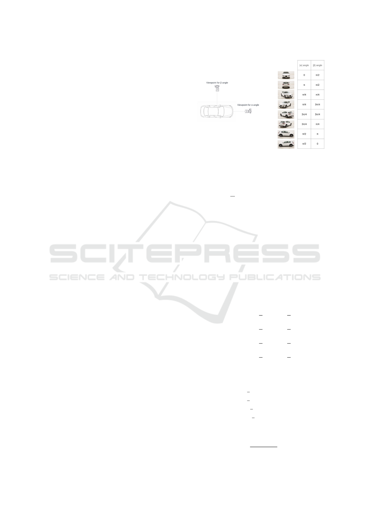
absolute values of two novel angles: α and β.

Alpha Discriminator (|α|). The α angle represents

the azimuthal view from the car’s front position.

Speciﬁcally:

• α = 0 depicts a direct frontal view of the car.

• α = π corresponds to a direct rear view.

• α = π/2 represents the left side view.

• α = −π/2 equates to the right side view.

Given the absolute interpretation |α|, it inherently

serves as a front/rear discriminator. However, this ab-

solute representation also forfeits its ability to distin-

guish between the car’s left and right sides.

Beta Discriminator (|β|). The β angle complements

α and serves a similar function but with different ref-

erence points:

• β = 0 signiﬁes the car’s left side (driver’s seat)

view.

• β = π corresponds to the car’s right side (passen-

ger seat) view.

• β = π/2 indicates the car’s rear view.

• β = −π/2 represents the direct frontal view.

Being an absolute representation |β|, it naturally

acts as a left/right discriminator, but similarly loses

distinction between front and rear views.

A visualization is provided to elucidate these an-

gles and their orientation in Figure 3.

Loss Function. The network optimizes a composite

loss function derived from the binary cross-entropy

(BCE) loss for both α and β predictions. Formally,

the loss L is given by:

L = BCE(α

pred

,α

true

) + BCE(β

pred

,β

true

), (4)

Figure 3: On the left: viewpoints visualization for the α and

β angles. On the right: Viewpoint of a car and correspond-

ing values of |α| and |β|.

where the binary cross-entropy (BCE) is deﬁned as:

BCE(y, ˆy) = −

∑

i=1

log( ˆy

) + (1 − y

)log(1 − ˆy

)],

(5)

where y represents the true labels (ground truths), ˆy

denotes the predicted values from the network, and N

is the total number of samples.

Azimuth Calculation from the Sigmoids

Predictions. To estimate the azimuth ϕ from

the sigmoid outputs, it is necessary to transform these

outputs to angles within the range [0, π].

abs

,β

abs

= y

sigmoids

× π (6)

Here, α

abs

and β

abs

represent the absolute angles

corresponding to the front/rear and left/right discrim-

inators, respectively. The next step is to determine the

speciﬁc quadrant of the azimuth angle based on the

values of α

abs

and β

abs

↔ α

abs

∧ β

abs

, (7)

↔ α

abs

≥

∧ β

abs

, (8)

↔ α

abs

≥

∧ β

abs

≥

, (9)

↔ α

abs

∧ β

abs

≥

. (10)

Having determined the quadrant, it is necessary

to compute the secondary angle, α

2,β

, based on the

quadrant and the value of α

abs

and β

abs

2,β











− β

abs

, if Q

+ β

abs

, if Q

− β

abs

, if Q

−

+ β

abs

, if Q

(11)

The mean angle,

α, is then computed by averaging

abs

and α

2,β

α =

abs

+ α

2,β

. (12)

VISAPP 2024 - 19th International Conference on Computer Vision Theory and Applications

856

Lastly, the azimuth ϕ is obtained by adjusting the

sign of

α based on the quadrant:

ϕ =

α × (−1)

δ(Q

∨Q

)

, (13)

where δ is the Kronecker delta function, which as-

signs a value of 1 if either condition Q

or Q

is true,

and 0 otherwise.

Drawbacks. The introduction of two discriminators

for azimuth representation can make the network’s

prediction mechanism less intuitive and more intricate

than the more direct sin-cos representation. More-

over, by utilizing absolute values and conﬁning out-

puts to the range [0, π], there is potential for a loss

of precision in angle estimation, especially when the

real angle hovers near the deﬁned boundaries.

4.3 Evaluation Method

Viewpoint estimation, especially for automobile ori-

entation, distinguishes itself from traditional classiﬁ-

cation tasks by predicting a continuous variable in-

stead of categorical outputs. In this work, by de-

composing the target into two variables (e.g., sin/cos

or alpha/beta), it is possible to employ classical re-

gression error metrics for evaluation. Therefore, be-

sides the commonly used Median Error (MedErr) and

Accuracy within π/6 (Acc

π/6

), regression evaluation

metrics like Mean Absolute Error (MAE), Root Mean

Square Error (RMSE), and the coefﬁcient of determi-

nation (R

) have been incorporated, given their signif-

icance in assessing models yielding continuous pre-

dictions.

4.4 Training

4.4.1 Data Preparation

Dataset Split. The PASCAL3D+ dataset, which

was employed for this research, inherently provides

a train/validation split. The total number of images

in the dataset amounts to 5,475. Of these, 2,763 be-

long to the training set, while 2,712 are earmarked for

validation, representing a nearly even 50/50 split.

Data Augmentation. To boost the robustness of the

trained models and to mitigate overﬁtting, an array of

data augmentation techniques was integrated into the

pipeline:

• Rotation. Images were rotated with a random an-

gle constrained to a maximum of 10

◦

• Barrel/Pincushion Distortions. These were intro-

duced to simulate lens distortions.

• Brightness and Contrast Adjustments. Random

adjustments were made to image brightness and

contrast levels.

• Horizontal Flips. Images were horizontally

ﬂipped. It is essential to note that the azimuth an-

gle needs adjustment when ﬂipping.

Azimuth Adjustment for Horizontal Flips. When

an image is ﬂipped horizontally in the Sin-Cos ap-

proach, the sine value of the azimuth changes its sign

while the cosine value remains the same. Given the

original pose [sin(ϕ),cos(ϕ)], the adjusted pose after

a horizontal ﬂip becomes:

[ −sin(ϕ), cos(ϕ) ]. (14)

In the Directional Discriminators approach, the

value for α remains unchanged after the horizontal

ﬂip, but the value for β is subtracted from 1. Given

the original pose [α,β], the adjusted pose post hori-

zontal ﬂip becomes:

[ α, 1 − β ]. (15)

Network Backbone. For the neural network back-

bone, the EfﬁcientNetB0 architecture (Tan and

Le, 2019) was chosen, pre-trained on ImageNet

dataset (Russakovsky et al., 2015). EfﬁcientNetB0

is acknowledged for delivering state-of-the-art perfor-

mance while maintaining a relatively compact model

size. Its design philosophy makes it an ideal choice

for this research, ensuring efﬁcient training without

compromising accuracy.

4.4.2 Training Parameters & Hardware

Conﬁguration

The training process was governed by the following

parameters:

• Learning Rate: 5 × 10

−3

;

• Optimizer: Adam;

• Learning Rate Decay: 0.96;

• Batch Size: 32.

The models were trained for a maximum of 50

epochs. However, an early stopping mechanism was

integrated to halt training if the validation perfor-

mance did not improve for 7 consecutive epochs (pa-

tience parameter).

The training was facilitated on a hardware setup

and efﬁcient computation throughout the training pro-

cess.

Vehicle Pose Estimation: Exploring Angular Representations

857

5 RESULTS

5.1 Quantitative Results

The quantitative assessment of the viewpoint estima-

tion performance comprises two tables. Table 1 pro-

vides a detailed performance evaluation of the pro-

posed methods using all ﬁve metrics—Median Error,

Accuracy within π/6, Mean Absolute Error (MAE),

Root Mean Square Error (RMSE), and R

. In con-

trast, Table 2 exclusively compares the proposed

methodologies on the PASCAL3D+ category-speciﬁc

viewpoint estimation for cars with several state-of-

the-art methods using the two metrics that are widely

reported in existing literature.

Table 1: Comprehensive Performance Metrics for View-

point Estimation Methods.

Approach MAE RMSE R

Acc

π/6

MedErr

Sin-Cos 7.3 14.8 0.95 0.97 3.5

Directional Discriminators 7.2 14.5 0.95 0.97 3.4

• Comprehensive Performance Assessment. Ta-

ble 1 showcases the full breadth of performance

metrics for both of the described methodologies.

The Directional Discriminators approach demon-

strates a slightly superior performance with an

MAE of 7.2, RMSE of 14.5, and R

of 0.95. In

comparison, the Sin-Cos representation achieves

an MAE of 7.3, RMSE of 14.8, and an equivalent

score of 0.95.

• Benchmark Achievement. Both of the presented

methodologies—the Sin-Cos representation and

the Directional Discriminators approach — sur-

pass all the prior methods documented. Remark-

ably, both of the described methods reach an

Acc

π/6

score of 0.97, which stands as the top per-

formance among the evaluated techniques. Fur-

ther emphasizing the accuracy of the proposed

methods, the MedErr metric—which gauges the

median error—registers its lowest values for the

discussed approaches. The Directional Discrim-

inators leads with a MedErr of 3.4, closely fol-

lowed by the Sin-Cos representation at 3.5.

• Intra-Comparison of the Two Approaches. A

side-by-side examination of the two techniques

reveals closely aligned results. The Directional

Discriminators slightly outperforms the Sin-Cos

representation in terms of MedErr. Nonetheless,

the difference is a mere 0.1, which, in practical

applications, might fall within an acceptable mar-

gin of error. This tight competition underscores

the robustness and reliability of both approaches.

• Residuals Analysis. One powerful diagnostic

tool to assess the accuracy and reliability of the

viewpoint prediction model is to inspect the dis-

tribution of residuals — the differences between

the observed orientations and their predicted val-

ues. For a given true orientation ϕ and its pre-

dicted orientation

ϕ, the residual r is given by:

r = ϕ −

ϕ. (16)

The histogram of residuals for the Directional

Discriminators, shown in Table 4 approach re-

veals a compellingly centered distribution around

0, indicating a generally accurate prediction by

the model.

However, the presence of non-zero residuals in

extreme intervals such as r < −150

◦

and r > 150

◦

signiﬁes occasional outlier predictions. These

outliers emphasize that, despite the model’s over-

all strong performance, there remains room for

further reﬁnement. Such sporadic, signiﬁcantly

erroneous predictions underscore the need for on-

going research to perfect the model and minimize

these anomalies.

Table 2: Results on PASCAL3D+ category-speciﬁc view-

point estimation (car). Acc

π/6

measures accuracy (the

higher the better) and MedErr measures error (the lower the

better).

Method Acc

π/6

MedError

(Prokudin et al., 2018) 0.91 4.5

(Su et al., 2015) 0.88 6.0

(Mousavian et al., 2017) 0.90 5.8

(Tulsiani and Malik, 2015) 0.90 8.8

(Pavlakos et al., 2017) - 5.5

(Grabner et al., 2018) 0.94 5.1

3DPoseLite (Dani et al., 2021) 0.92 -

(Xiao et al., 2019) 0.91 5.0

(Klee et al., 2023) - 4.9

(Nie et al., 2020) 0.92 5.1

(Mahendran et al., 2018) 0.95 4.5

Ours (Sin-Cos) 0.97 3.5

Ours (Directional Discriminators) 0.97 3.4

Figure 4: Residuals distribution for the Directional Dis-

criminators approach.

VISAPP 2024 - 19th International Conference on Computer Vision Theory and Applications

858

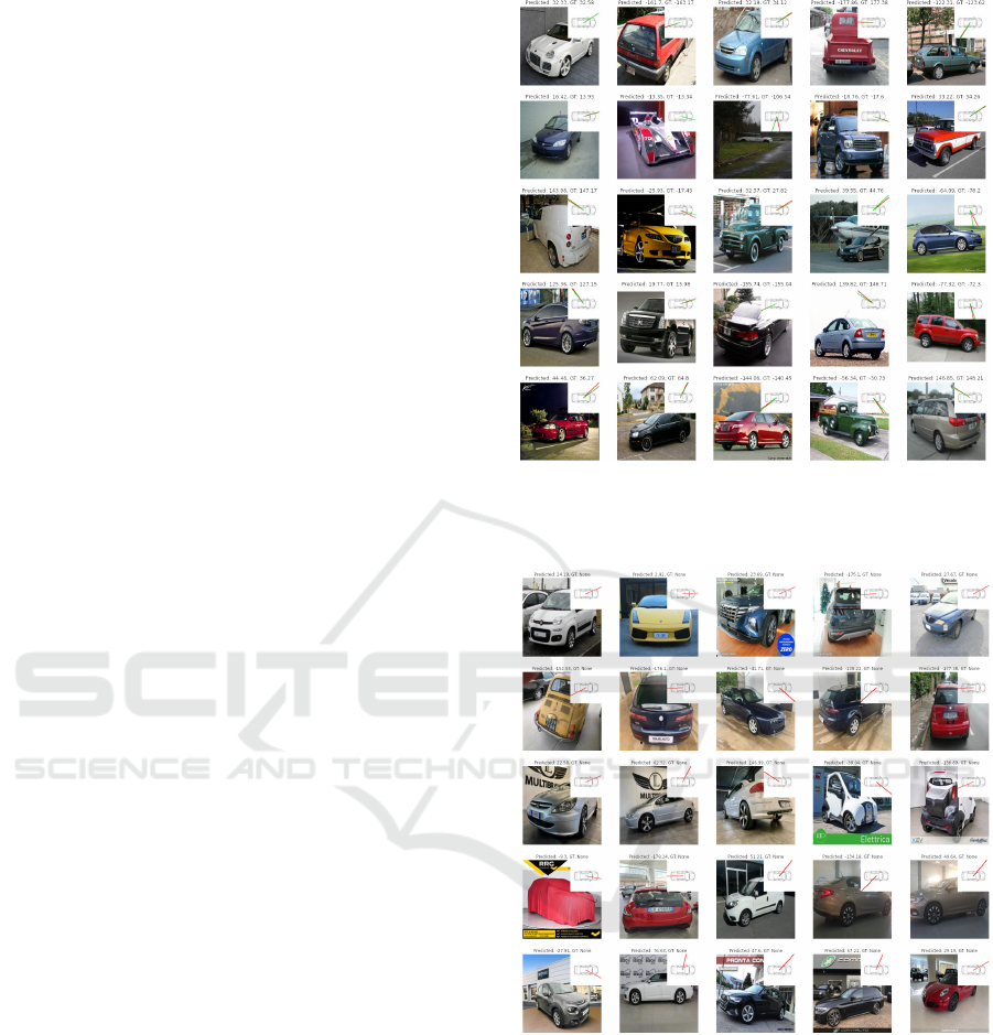
5.2 Qualitative Results

PASCAL3D+ Validation Set. Figure 5 presents a

5 × 5 grid showcasing predictions made on the vali-

dation set of the PASCAL3D+ dataset. Each image in

this grid is accompanied by an azimuth diagram sit-

uated at the right top corner, in which the predicted

azimuth is marked with a red line while the ground

truth is indicated by a green line. A closer inspection

of the images reveals the striking proximity between

the predicted and actual orientations across the major-

ity of samples, highlighting the model’s effectiveness.

However, it is essential to recognize instances like

the sample in the second row and third column where

the divergence between the prediction and the ground

truth is nearly 30

◦

. Contrary to initial impressions,

this deviation does not necessarily reﬂect an inaccu-

racy in the model. Upon closer inspection, it becomes

evident that the ground truth provided for this partic-

ular image does not align seamlessly with the actual

orientation of the car, hinting at occasional noise and

inconsistencies in the PASCAL3D+ dataset. Such ob-

servations underline the importance of maintaining a

critical approach when evaluating predictions, espe-

cially in the context of potentially noisy datasets.

Internet-Sourced Images. The versatility and gen-

eralizability of the proposed model are further demon-

strated in Figure 6. This ﬁgure showcases a 5 ×5 grid

of car images sourced from the internet, beyond the

boundaries of the PASCAL3D+ dataset. As these im-

ages come without any associated ground truth, only

the predicted azimuth, denoted by a red line, is illus-

trated on the azimuth diagrams. Notably, even in the

absence of ground truth for comparison, the predic-

tions appear highly plausible, resonating well with the

visual orientations of the cars.

An intriguing observation from this set is the im-

age located in the ﬁrst column and fourth row, where a

car is obscured by a car cover. Despite this blanket ob-

scuring the intricate details and distinctive features of

the vehicle, the model still manages to deduce the az-

imuth quite accurately. This exempliﬁes the model’s

ability to generalize and make predictions based on

broad contextual cues, even when faced with uncon-

ventional scenarios.

Model Interpretability and Utility. Visual results,

as presented in the aforementioned ﬁgures, are vital

for offering an intuitive sense of model performance.

They not only establish conﬁdence in the model’s

quantitative metrics but also showcase its utility in

real-world, diverse scenarios. Moreover, such qualita-

tive results facilitate potential troubleshooting and re-

Figure 5: Sample predictions on the PASCAL3D+ valida-

tion set. Red and green lines on the azimuth diagrams corre-

spond to predicted and ground truth azimuths, respectively.

Figure 6: Sample predictions on car images sourced from

the internet. Only the predicted azimuth (red line) is de-

picted due to the absence of ground truth.

ﬁnement strategies by revealing situations where the

model might underperform or when external factors,

like dataset noise, come into play.

6 CONCLUSIONS

This study has introduced two methods for car az-

imuth estimation, utilizing the sinusoidal properties

Vehicle Pose Estimation: Exploring Angular Representations

859

of orientations and directional discriminators. Both

methods demonstrated state-of-the-art performance

on the PASCAL3D+ dataset, with minimal perfor-

mance differences under certain conditions, high-

lighting their practical applicability.

In terms of potential improvements, exploring a

range of data augmentation techniques could enhance

model robustness, particularly in real-world scenar-

ios. Additionally, accuracy might be further reﬁned

by employing model ensembling to combine predic-

tions from various models or iterations, thereby re-

ducing the impact of outlier predictions.

ACKNOWLEDGMENTS

This work was partially supported by the MUR under

the grant “Dipartimenti di Eccellenza 2023-2027” of

the Department of Informatics, Systems and Commu-

nication of the University of Milano-Bicocca, Italy.

REFERENCES

Beyer, L., Hermans, A., and Leibe, B. (2015). Biternion

nets: Continuous head pose regression from discrete

training labels. In German Conference on Pattern

Recognition, pages 157–168. Springer.

Buzzelli, M. and Segantin, L. (2021). Revisiting the

compcars dataset for hierarchical car classiﬁcation:

New annotations, experiments, and results. Sensors,

21(2):596.

Dani, M., Narain, K., and Hebbalaguppe, R. (2021).

3DPoseLite: A compact 3D pose estimation using

node embeddings. In Proceedings of the IEEE/CVF

Winter Conference on Applications of Computer Vi-

sion, pages 1878–1887.

David, L. (2004). Distinctive image features from scale-

invariant keypoints. International journal of computer

vision, 60:91–110.

Felzenszwalb, P. F. and Huttenlocher, D. P. (2005). Pic-

torial structures for object recognition. International

journal of computer vision, 61:55–79.

Geiger, A., Lenz, P., and Urtasun, R. (2012). Are we ready

for autonomous driving? The KITTI vision bench-

mark suite. In IEEE conference on computer vision

and pattern recognition.

Grabner, A., Roth, P. M., and Lepetit, V. (2018). 3D

pose estimation and 3D model retrieval for objects in

the wild. In Proceedings of the IEEE conference on

CVPR, pages 3022–3031.

He, K., Gkioxari, G., Doll

ar, P., and Girshick, R. (2017).

Mask R-CNN. In Proceedings of the IEEE ICCV,

pages 2961–2969.

Kendall, A., Grimes, M., and Cipolla, R. (2015). Posenet: A

convolutional network for real-time 6-DoF camera re-

localization. In Proceedings of the IEEE international

conference on computer vision, pages 2938–2946.

Klee, D. M., Biza, O., Platt, R., and Walters, R.

(2023). Image to sphere: Learning equivariant fea-

tures for efﬁcient pose prediction. arXiv preprint

arXiv:2302.13926.

Lepetit, V., Moreno-Noguer, F., and Fua, P. (2009). Ep n

p: An accurate o (n) solution to the p n p problem.

International journal of computer vision, 81:155–166.

Mahendran, S., Lu, M. Y., Ali, H., and Vidal, R. (2018).

Monocular object orientation estimation using Rie-

mannian regression and classiﬁcation networks. arXiv

preprint arXiv:1807.07226.

Mousavian, A., Anguelov, D., Flynn, J., and Kosecka, J.

(2017). 3D bounding box estimation using deep learn-

ing and geometry. In Proceedings of the IEEE con-

ference on Computer Vision and Pattern Recognition,

pages 7074–7082.

Nie, W.-Z., Jia, W.-W., Li, W.-H., Liu, A.-A., and Zhao,

S.-C. (2020). 3D pose estimation based on reinforce-

ment learning for 2D image-based 3D model retrieval.

IEEE Transactions on Multimedia, 23:1021–1034.

Pavlakos, G., Zhou, X., Chan, A., Derpanis, K. G., and

Daniilidis, K. (2017). 6-DoF object pose from seman-

tic keypoints. In 2017 IEEE international conference

on robotics and automation, pages 2011–2018.

Prokudin, S., Gehler, P., and Nowozin, S. (2018). Deep di-

rectional statistics: Pose estimation with uncertainty

quantiﬁcation. In Proceedings of the European con-

ference on computer vision (ECCV), pages 534–551.

Qin, Z., Wang, J., and Lu, Y. (2019). Monogrnet: A geo-

metric reasoning network for monocular 3D object lo-

calization. In Proceedings of the AAAI Conference on

Artiﬁcial Intelligence, volume 33, pages 8851–8858.

Russakovsky, O., Deng, J., Su, H., Krause, J., Satheesh, S.,

Ma, S., Huang, Z., Karpathy, A., Khosla, A., Bern-

stein, M., et al. (2015). Imagenet large scale visual

recognition challenge. International journal of com-

puter vision, 115:211–252.

Srivastava, N., Hinton, G., Krizhevsky, A., Sutskever, I.,

and Salakhutdinov, R. (2014). Dropout: a simple way

to prevent neural networks from overﬁtting. The jour-

nal of machine learning research, 15(1):1929–1958.

Su, H., Qi, C. R., Li, Y., and Guibas, L. J. (2015). Render

for cnn: Viewpoint estimation in images using cnns

trained with rendered 3D model views. In Proceedings

of the IEEE international conference on computer vi-

sion, pages 2686–2694.

Tan, M. and Le, Q. (2019). Efﬁcientnet: Rethinking model

scaling for convolutional neural networks. In Interna-

tional conference on machine learning, pages 6105–

6114. PMLR.

Tulsiani, S. and Malik, J. (2015). Viewpoints and keypoints.

In Proceedings of the IEEE Conference on Computer

Vision and Pattern Recognition, pages 1510–1519.

Xiang, Y., Mottaghi, R., and Savarese, S. (2014). Beyond

pascal: A benchmark for 3D object detection in the

wild. In IEEE winter conference on applications of

computer vision, pages 75–82. IEEE.

Xiao, Y., Qiu, X., Langlois, P.-A., Aubry, M., and Marlet, R.

(2019). Pose from shape: Deep pose estimation for ar-

bitrary 3D objects. arXiv preprint arXiv:1906.05105.

VISAPP 2024 - 19th International Conference on Computer Vision Theory and Applications

860