Simultaneous Optimization of Edge Bundling and Node Layout Using

Genetic Algorithm

Junsei Meikari

and Ryosuke Saga

Graduate School of Humanities and Sustainable System Sciences, Osaka Prefecture University, Sakai, Japan

Graduate School of Informatics, Osaka Metropolitan University, Sakai, Japan

Keywords: Visualization, Edge Bundling, Node Layout, Genetic Algorithm.

Abstract: This paper describes an evolutionary visualization method that performs edge bundling during the execution

of the genetic algorithm. There are several node layout algorithms and edge bundling, however, there are no

methods considering both algorithms simultaneously. This paper proposes an algorithm to optimize the fitness

function of GABEB, which is genetic algorithm-based edge bundling, and Zhang’s node layout

simultaneously. The experiments for the sample graphs show the improved result from the viewpoints of

several evaluation criteria.

1 INTRODUCTION

The graph, consisting of edges representing

connections between nodes, is used to visually

represent various relationships among data

represented as nodes, such as in aviation charts or

relation diagrams (Saga 2012). However, as the scale

and complexity of the graph increase, it becomes

challenging for users to comprehend the relationships

between nodes, leading to visual clutter problem. To

address such issues, various visualization techniques

have been proposed over time, including force-

directed graph drawing (Kamada, 1989) and

compound graph layout (Sugiyama 1991)(Dogrusoz

2009).

In recent years, edge bundling has been proposed

as a method to solve visual clutter problem. Edge

bundling involves spatially grouping edges according

to certain rules, reducing the visual complexity of the

graph and making it easier to visually grasp the

connection relationships between nodes.

Various edge bundling techniques have been

proposed, and their effectiveness has been

demonstrated (Lhuillier 2017). On the other hand, in

recent years, stochastic optimization approaches such

as Genetic Algorithms (GA) have also been

implemented to address these problems. The

advantages of using such GA approaches include the

potential for obtaining visualization results not

https://orcid.org/0000-0003-1528-6534

anticipated by humans and the ability to apply

stochastic optimization methods regardless of the

continuity of the visualization problem space.

The studies like Ferreira et al. (Ferreira 2018) and

Saga et al. (Saga 2020) have proposed edge bundling

using GA, receiving certain evaluations. While

various edge bundling techniques have been proposed,

those that include the process of adjusting node

positions in the edge bundling process have been

rarely suggested. When the process of adjusting node

positions is not included in edge bundling techniques,

even if the method effectively bundles edges before

application, the visualization effects of edge bundling

may not be fully realized due to the inappropriate

positions of nodes in the graph before the application

of the method, especially in cases with a high number

of edge crossings.

Considering the aspects, Meikari et al. (Meikari

2022) proposed an initial approach to simultaneously

optimize node layout and edge bundling using a

genetic algorithm. However, the solution to the

algorithm is the position of the nodes and the

combination of edges for bundles, and actual edge

bundling takes place after the completion of the

genetic algorithm. Therefore, the process of bundling

edges and node layout can be considered separate.

In this paper, our goal is to propose an

evolutionary visualization method where node layout

and edge bundling are optimized simultaneously.

Meikari, J. and Saga, R.

Simultaneous Optimization of Edge Bundling and Node Layout Using Genetic Algorithm.

DOI: 10.5220/0012574200003660

Paper published under CC license (CC BY-NC-ND 4.0)

In Proceedings of the 19th International Joint Conference on Computer Vision, Imaging and Computer Graphics Theory and Applications (VISIGRAPP 2024) - Volume 1: GRAPP, HUCAPP

and IVAPP, pages 741-748

ISBN: 978-989-758-679-8; ISSN: 2184-4321

741

Additionally, we aim to validate the visualization

effects of this method by running the implemented

program and comparing the obtained results with

those of the methods by Meikari’s method.

2 RELATED WORKS

2.1 Edge Bundling

Edge bundling is a graph visualization technique that

involves spatially grouping edges within a graph

according to certain rules. This bundling aims to

reduce the visual clutter of the graph, making it easier

to visually comprehend the connection relationships

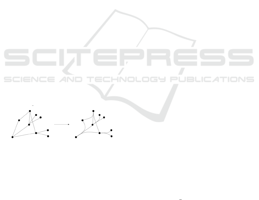
between nodes connected by edges. Figure 1

illustrates an example of a graph with edge bundling.

Originating in 1989 with the simplification of

graph edges through spatial concentration (Newbery

1989), edge bundling has evolved into various

methods such as Hierarchical Edge Bundling (Holten

2006) and others, demonstrating its effectiveness

(Telea, 2010) (Ersoy, 2011) (Hurter, 2012) (Cui,

2008) (Lhuillier, 2017). Another well-known method

is Force-Directed Edge Bundling (FDEB), proposed

by Holten et al. (Holten, 2009). FDEB employs a

mechanical approach, modeling edges as springs that

attract each other. It evenly allocates splitting points

along the edges, calculates the magnitude and

direction of forces acting on each splitting point based

on the distance between points and the geometric

similarity between edges, and forms smooth curves

through iterative movements of splitting points and

information updates.

Figure 1: Edge Bundling.

2.2 Edge Bundling Using Genetic

Algorithm

In recent years, probabilistic optimization approaches

such as Genetic Algorithms (GA) have been

implemented. The benefits of using such approaches

include the potential to obtain visualization results not

anticipated by humans and the ability to apply

stochastic optimization methods regardless of

whether the visualization problem space is

continuous. Additionally, there is an implementation

advantage in terms of ease.

Evolutionary Edge Bundling (EEB), proposed by

Ferreira et al. (Ferreira 2018), is an edge bundling

method that utilizes genetic algorithms to determine

bundles (sets of edges) that should be grouped

together. Therefore, the process of bundling edges is

not included in the genetic algorithm's process, and

the actual bundling process uses FDEB after the

genetic algorithm concludes. The graph is evaluated

based on the similarity in angle and length of edges

within bundles that should be maximized and the

number of bundles that should be minimized.

Evolutionary Node Layout and Edge Bundling

(ENLEB), proposed by Meikari et al. (Meikari 2022),

integrates EEB and node layout methods into a single

genetic algorithm. This was the first approach aiming

to simultaneously optimize edge bundling and node

layout in evolutionary visualization. Therefore, it

allows obtaining visualization effects considering

both edge bundling and node layout. The solution

obtained by ENLEB includes the positions of nodes

and bundles of edges, and similar to EEB, the process

of bundling edges using FDEB occurs after the

genetic algorithm concludes. Hence, the processes of

node layout and edge bundling are executed

separately.

Genetic Algorithm Based Edge Bundling

(GABEB), proposed by Saga et al. (Saga 2020), is an

edge bundling method that uses genetic algorithms by

placing control points on edges and optimizing their

positions. Control point movements are treated as

genes, and genetic operations such as crossover and

mutation are applied. The evaluation of individuals

includes four aesthetic criteria related to edge

bundling: Mean Edge Length Difference (MELD),

Mean Occupation Area (MOA), Edge Density

Distribution (EDD) proposed by Saga et al.(Saga

2016), and Path Quality proposed by Cui et al. (Cui

2008).

2.2.1 Mean Edge Length Difference

Mean Edge Length Difference (MELD) is a criterion

to express the difference from the original edges after

edge bundling. A smaller change of edge lengths

indicates superior edge bundling because of over-

bundling, whereas a large change often leads to a loss

of the meaning of the original network. MELD is

calculated as

𝑀𝐸𝐿𝐷





∑ |

𝐿





𝑒



−𝐿



𝑒

|

∈

)

where n is the number of edges, E is the edge set, and

L(e) and L’(e) are the lengths of edge e before and

after edge bundling, respectively. In our approach, we

aim to minimize the MELD.

IVAPP 2024 - 15th International Conference on Information Visualization Theory and Applications

742

2.2.2 Mean of Occupation Area

Mean of Occupation Area (MOA) indicates the

degree among the compressed areas before and after

edge bundling. Based on the idea that better bundling

can compress the area occupied by the edges, MOA

is calculated as

𝑀𝑂𝐴=

𝑁



𝑂



𝑒





∈



(2)

where N is the number of total areas, O(e) is the set of

areas occupied by edge e based on an occupation

degree (we use 5% of unit area), and | | indicates the

number of elements contained by a set. Minimising

the MOA is one of our optimization goals.

2.2.3 Edge Density Distribution

Edge Density Distribution (EDD) is rooted in the idea

that a better edge bundling method can gather edges

within a unit area and that the density per unit is high.

EDD is calculated as

𝐸𝐷𝐷=



||

∑

𝐻



𝑝



−𝐻





∈

(3)

where P is a set of pixels, H(p) is the number of edges

pathing pixel p, and H is the average of H(p). We aim

to maximise the EDD.

2.2.4 Path Quality

Path Quality (PQ) expresses the degree of zigzag. The

lower the PQ, the better the edge bundling. PQ is

calculated by the summation of angle differences

between neighbours as

with

∆





𝐴



−𝐴



𝐴



−𝐴



−2𝜋

2𝜋+

𝐴



−𝐴



−𝜋<

𝐴



−𝐴



< 𝜋

𝐴



−𝐴



> 𝜋

𝐴



−𝐴



< −𝜋

(5)

and

𝛾



= 

sign



∆





=sign



∆





sign



∆





≠sign



∆





(6)

, where m is the number of segments divided by

control points+1, and A

is the angle between the

original edge and the segment edge. In our GA, we

try to maximize PQ. We use the above four criteria

separately and perform multi-objective optimization.

3 PROPOSED METHODS

In this paper, we address the issue present in EEB,

where the processes of edge bundling and node layout

were executed separately. We propose an

evolutionary visualization method that

simultaneously performs edge bundling and node

layout while optimizing both using a genetic

algorithm. To achieve this, we integrate the genetic

algorithm-based edge bundling method GABEB and

Zhang et al.'s node layout method (Zhang 2005) into

a single genetic algorithm.

The reason for using GABEB is that it operates as

a genetic algorithm solely for manipulating control

points on edges, without considering the impact on

node positions. This makes it less likely to encounter

problems when simultaneously performing node

layout and edge bundling. In the context of our

method aiming to perform edge bundling and node

layout concurrently, GABEB is well-suited for

conducting edge bundling within the genetic

algorithm.

Additionally, we choose Zhang et al.'s node layout

method for two main reasons. First, it is a genetic

algorithm-based node layout method. Second, by

adjusting the weights of the evaluation function in

Zhang et al.'s method, our proposed method can more

easily reflect elements such as the number of edge

crossings that need improvement in the graph

evaluation, especially in the node layout part.

3.1 The Process of Genetic Algorithm

Figure 2 illustrates the flow of the genetic algorithm

for this method. The genetic algorithm of this method

repeats the process of crossover, mutation, joining,

individual evaluation after generating the initial

individuals, and generation update until the

termination condition is satisfied. When a control

point is subject to crossover or mutation, if the control

point is bound to one of the other control points, it is

unbound to prevent an anomaly in the information on

the movement of the control point.

Figure 2: Process of Generic Algorithm.

Generate Initial Population

Evaluate population

Crossover, Mutation

Join Control Points

Update Generation

Unjoin Control Points

𝑃𝑄=



−



𝛾



∆















∈



(4)

Simultaneous Optimization of Edge Bundling and Node Layout Using Genetic Algorithm

743

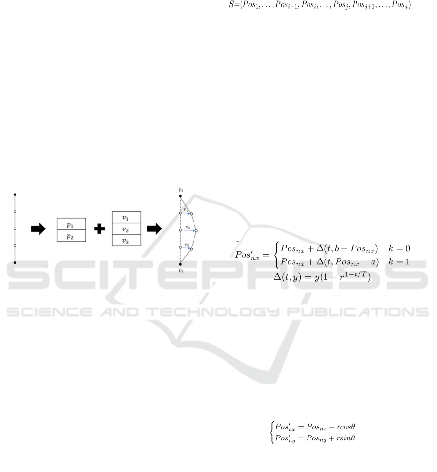
3.2 Chromosomes

Figure 3 shows an image of the individual

representation of the method. Based on GABEB, the

individual representation incorporates the concept of

control points in FDEB. In FDEB, edges are equally

divided by the number of control points, and edge

bundling is performed by moving control points

based on calculations based on mechanical rules such

as the distance between control points. In contrast,

GABEB treats the amount of movement of each

control point as a gene, which represents each

individual. As in FDEB, the original positions of the

control points are assumed to be equally divided by

the number of control points. In addition to the

information on the amount of control point movement

for edge bundling, this method also treats the node

position of each edge as a gene for the purpose of

node layout.

Figure 3: Genetic Representation.

3.3 Crossover

The crossover is performed with respect to the

operation on the position of a node and the amount of

movement of the control point of an edge. For the

former, a simple crossover is performed, in which the

position of one node is exchanged between two parent

individuals, and an inversion, in which the position of

a node of one parent is manipulated. For the latter

operation on the mobility of the control point, we

perform the blended crossover (BLX-α) (α=0.5)

(Eshelman 1993).

The inversion of this method is an operation to

change the position of a node by numbering the

collected positions of the nodes at both ends of an

individual edge, and then inverting the numbers

within a randomly set interval of numbers. Let S be

the list of node positions before applying inversion, S’

be the list of node positions after applying inversion,

i to j be the interval of node positions to be

manipulated, and Pos

be the collected node position

information, the operation by inv ersion is as in

quations (7) and (8). After the crossover is applied to

the position of a node, the change in the position of

the node is reflected in the entire gene. Each

crossover is assigned an independent crossover

probability.

)

𝑆ʹ = 𝑃𝑜𝑠

,...,𝑃𝑜𝑠

1

, 𝑃𝑜𝑠



, 𝑃𝑜𝑠

1

,..,

𝑃𝑜𝑠

1

, 𝑃𝑜𝑠



, 𝑃𝑜𝑠

1

,...,𝑃𝑜𝑠





)

3.4 Mutation

Mutation involves two genetic manipulations to

change the position of the node as indicated by the

node layout method of Zhang et al. and one genetic

manipulation to change the amount of movement of

the control point.

The mutations shown by Zhang et al. include non-

uniform mutation, in which the shift of node position

becomes smaller with each generation, and single-

vertex-neighbourhood mutation, in which the

position shifts within a circular range from the

original node position.

Let Pos

be the X-coordinate of the nth node of

an individual and Pos

’ be the X-coordinate of the

node after the move, the shift of a node's position due

to non-uniform mutation is calculated by the

equations (9) and (10).

(9)

(10)

In this case, 𝑏 is the maximum value of the X-axis of

the set graph plotting range, and 𝑎 is its minimum

value. 𝑘 is a value of 0 or 1 randomly determined

each time, 𝑇 is the maximum number of generations,

and 𝑡 is the current number of generations. For the

sake of illustration, we have only described the

operation on the X coordinate, but the operation on

the Y coordinate is similar, and they are performed

simultaneously.

The shift of a node's position by single-vertex-

neighborhood mutation is calculated by the equations

(11) and (12).

(11)

𝑟= 𝑑



∗



1 −𝑡/𝑇



(12)

In this case, 𝜃 is randomly determined between 0 and

2π. And d

ideal

is calculated by





𝑠/𝑛



where s is the

area of the drawing area. As in crossover, after the

mutation on the node position is applied, the change

in node position is reflected in the whole gene.

Mutation of a control point is performed by

assigning a new random displacement to the target

control point that is less than the set maximum

displacement. The mutation probability for the

position of the node and the mutation probability for

the displacement of the control point are assigned

IVAPP 2024 - 15th International Conference on Information Visualization Theory and Applications

744

independent mutation probabilities. When it is

decided that a mutation on the node position is to be

made, one mutation is made at random among the two

mutations.

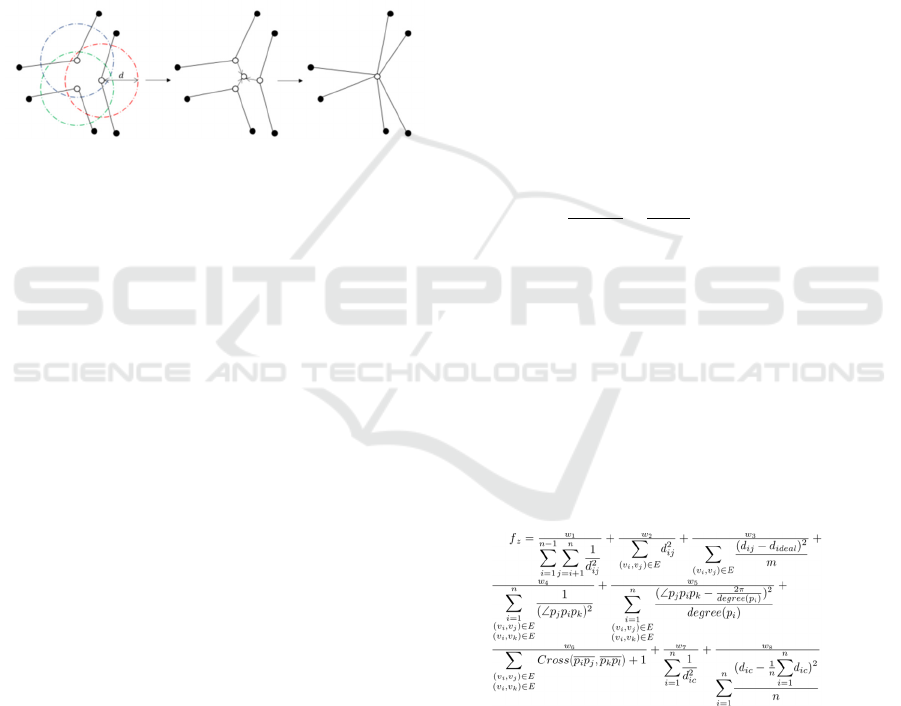
3.5 Control Points Joining

To alleviate the problem of insufficient edge bundling

because control points that existed in GABEB rarely

exist at the same coordinates, the join operation,

which places control points that are close enough

together at exactly the same coordinates(Saga 2023).

The join process of the control points is performed by

the following process (Figure 4).

Figure 4: Join process of control points.

1. Find all control points in each edge for which the

distance between control points is less than or

equal to the set distance (d) that admits a join,

and for which no other control points of the edge

containing the joined control points are joined to

any of the control points.

2. The pair of control points with the shortest

distance between them is first joined. If a pair of

control points that has been joined before has an

edge in common, the pair is not joined.

3. Calculate the average coordinate of each set of

control points for which the coupling has been

determined and assign the amount of movement

from the reference point of the control point to

the average coordinate as the amount of

movement of each control point. In such a case,

the amount of movement before the coupling is

stored for use when the coupling is released.

If a control point that is subject to crossover and

mutation in edge bundling or a control point whose

edge contains a node that is subject to crossover and

mutation in node layout is bound to another control

point, the binding is unbundled. The reason for not

performing the crossover and mutation operation

while the control points are still joined is to prevent

any of the joined control points from moving beyond

an acceptable distance from the edge containing the

control point or node position due to the crossover or

mutation, which would cause visual confusion.

The unjoin of the control points between two

points is done by assigning to each control point the

amount of movement before the coupling was

performed. To unjoin two or more control points,

only the control points that have been subject to

crossover or mutation are assigned the amount of

movement before the join, and a new join is processed

for the remaining control points, starting from the

position of the control points before the join.

3.6 Fitness Function

The fitness function f of this method (equation (13))

is the sum of 𝑓



, which measures the quality of edge

bundling with reference to the individual evaluation

index used in GABEB, and the evaluation function f

shown in the node layout method by Zhang et al.

where 𝑤

and 𝑤

are weights for each evaluation

function.

𝑓

= 𝑤



𝑓



+ 𝑤



𝑓



(13)

The fitness function for edge bundling f

is the

sum of the values for edge bundling used in GABEB:

EDD and PQ should be maximized, but MELD and

MOA should be minimized, so the inverse is taken for

these two values.

𝑓



𝑀𝐸𝐿𝐷

𝑀𝑂𝐴

+ 𝐸𝐷𝐷+ 𝑃𝑄

(14)

The fitness function (equation (15)) presented in

the node layout method of Zhang et al. provides an

aesthetic evaluation of node locations and the edges

affected by them. Here, d

is the distance between

nodes p

and p

, 𝐸 is the entire set of edges, and m is

the number of edges. Also, ∠𝑝



𝑝



𝑝



 is the angle

between the edge with p

and the edge with p

that

share node p

, degree(p

) is the degree of node p

. And

is the distance between the location of the center

of the drawing area and node p

. Finally, w

is a weight

that the user can set to emphasize any aesthetic

feature.

(15)

Each term with these symbols of the equation (15)

has the following meaning. The first term increases as

the distance between nodes increases, and the second

term increases as the distance between edges

decreases. This prevents the distance between edges

from becoming too large while still evaluating low

node densities. The third term aims to unify the edge

lengths by bringing them closer to d

ideal

. The fourth

and fifth terms are evaluations of the angles between

Simultaneous Optimization of Edge Bundling and Node Layout Using Genetic Algorithm

745

edges and are intended to increase the angles between

edges and unify the angles between edges. The sixth

term, Cross(𝑝



𝑝





, 𝑝



𝑝





), is the value calculated by the

equation (16) and is intended to reduce the number of

edge crossings. Finally, the seventh and eighth terms

evaluate the symmetry of the graph.

(16)

3.7 Update and Termination

From the population that has undergone crossover

and mutation and the population of the current

generation, the top individuals are selected in a

number equal to the number of individuals in the

current generation to form the population of the next

generation. The termination condition is the

completion of the generation update for the set

maximum number of generations, or when the highest

evaluation value is not updated for 100 consecutive

generations.

3.8 Example

The parameters of the genetic algorithm used to

generate the examples are shown in Table1. The

parameters of the weights in 𝑓



are set to (0.02, 10, 1,

20, 200, 100000, 0.001, 1). The parameters are very

different from each other in order to equalize the

magnitude of each item's evaluation value. In

particular, the weight of 𝑤

is large, but this is because

the evaluation of crossing is treated low as the graph

scale increases, and because this method places

particular importance on the problem of edge crossing,

which cannot be solved by edge bundling. The

weights 𝑤



for the evaluation function of GABEB

and 𝑤



for the evaluation function of the node layout

method of Zhang et al. are set to 1, respectively.

Table 1: Parameters.

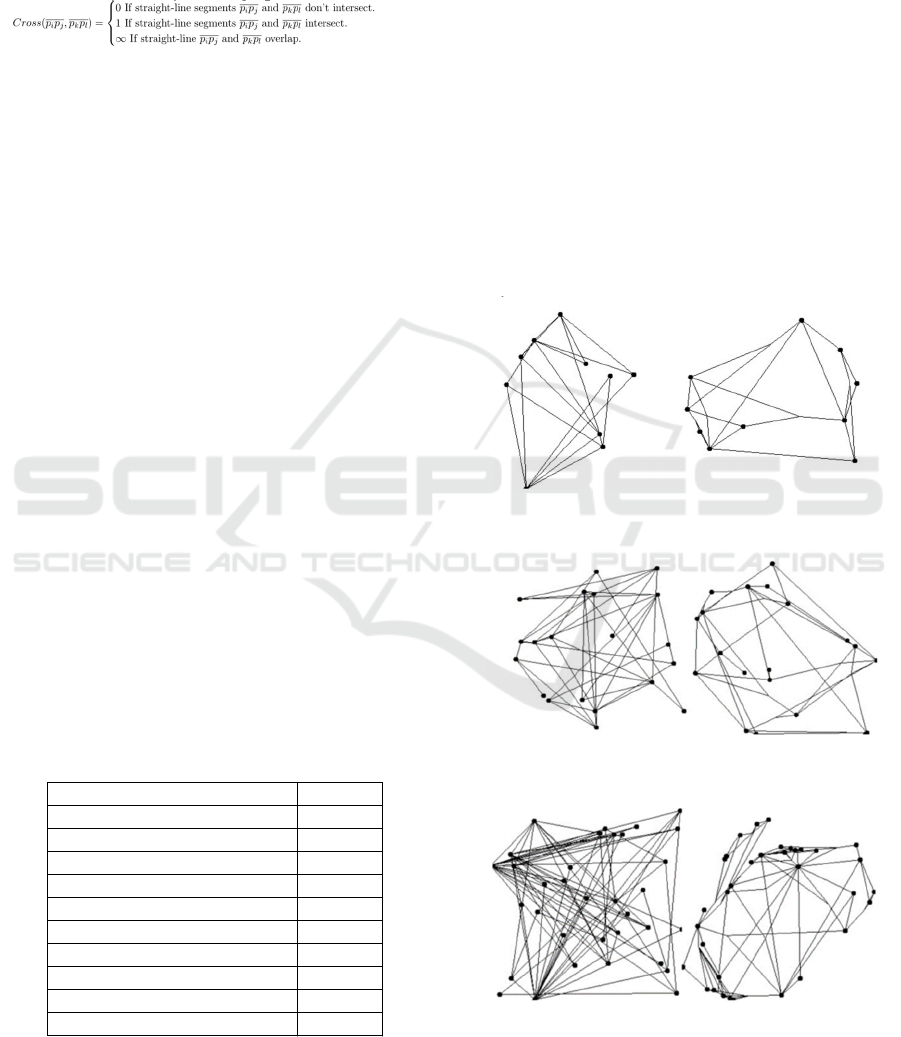
The graphs of Figure 5 to Figure 7 (the left are

examples of graphs before applied, and the graphs on

the right are examples after applied) show that the

effect of the parameter on the number of edge

crossings, which was set particularly high, is applied,

and the number of edge crossings is greatly reduced.

This is because the parameters for the evaluation

value that increases the distance between nodes and

the parameter for the evaluation value that unifies the

distance between nodes are set so large, depending on

the scale of the graph, that the other evaluation values

are not evaluated properly. This is because the

parameter setting prevents other evaluation values

from being evaluated appropriately because they

become very large depending on the scale of the

graph. In addition, the effect of edge bundling is not

so apparent in Figure 5 because the number of edges

is small and the effect of node layout is sufficient, but

in Figure 7, dense edges are bundled together in the

lower left corner and the effect of edge bundling is

fully shown.

Figure 5: An example applied to a graph with 10 nodes and

20 edges.

Figure 6: An example applied to a graph with 20 nodes and

40 edges.

Figure 7: An example applied to a graph with 34 nodes and

78 edges.

Parameters Value

Populations 100

Generations 100000

Crossover probability of Edge Bundlling 0.9

Mutation Probability of Edge Bundling 0.05

Crossover probability of node layout 0.75

Inversion probability of node layout 0.25

Mutation probability of node layout 0.25

Distance to allow coupling (d )10

Number of Control point 3

Length of one side of the MOA unit area 5

IVAPP 2024 - 15th International Conference on Information Visualization Theory and Applications

746

4 EXPERIMENTS

4.1 Environment

In order to compare the visualization effects with

ENLEB, the target graphs for the experiments were

the same as those used in the ENLEB experiments.

That is, randomly generated graphs G1 (10 nodes, 20

edges) and G2 (20 nodes, 40 edges), and three graphs

representing real world graphs G3 well-known as

karate club (34 nodes, 78 edges) (Zachary 1977), G4

as le miserable (62 nodes, 160 edges) (Girvan 2002),

G5 (77 nodes, 254 edges) (Knuth 1993) is the target

of this experiment. The criteria used for the

measurements were the same five aesthetic

evaluation criteria as in ENLEB. The evaluation

criteria are shown in Table 2, and the right column of

the table shows the desired results.

Table 2: Evaluation criteria.

In the experiments, the algorithm of the proposed

method was implemented and run on a PC with an

Intel Core i7-7500 3.4GHz CPU and 8 GB RAM. The

parameters of the genetic algorithm and fitness

function in the experiments are the same as those

shown in the application example of the proposed

method.

4.2 Result and Discussion

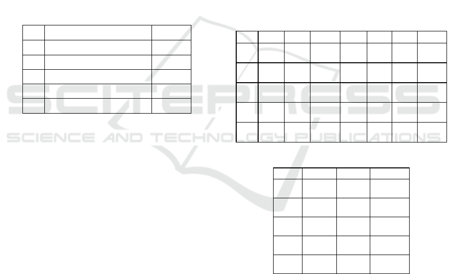
The results of the experiment are shown in Table 3.

The first row in each graph is for ENLEB, and the

second row is for this method. The results in Table 3

show that the symmetry of the graphs is consistently

improved compared to ENLEB.

For G1 to G3, where the graph scale is smaller,

there is an improvement in the number of edge

crossings (C1) and the similarity of the angles of the

edges in the bundle (C4). It can be attributed to the

positive effect of the inversion operation, which was

not implemented in ENLEB. On the other hand, the

deterioration in C2 and improvement in C4 can also

be attributed to the fact that the appropriate node

placement results in more opportunities for the

control points in the edges with high similarity to be

spatially close to each other, and less opportunities for

the control points in the edges that are not so close to

each other.

On the other hand, as the graph scale increased

like G4 and G5, the number of edge crossings (C1)

and the similarity of the angles (C3) and lengths of

the edges (C4) in the bundles deteriorated. The

number of bundles (C2) improved. The increase of C1

as the graph scale increases can be attributed to the

fact that the evaluation values other than the number

of edge crossings increased as the number of edges

and nodes increased, and the evaluation value for the

number of edge crossings was treated low, resulting

in insufficient optimization for C1. The change in C2

through C4 can also be attributed to the fact that as

C1 increases, control points in edges have more

opportunities to come closer together, resulting in

more bundling, but has also increased the chances of

bundling edges with low similarity between edges.

Table 3: Experimental results.

Table 4: Calculation Time(s).

The above results indicate that the number of edge

crossings, the similarity of the angles of the edges in

the bundles, and the symmetry of the graphs

improved for small-scale graphs, but as the scale

increased, the number of edge crossings increased,

which had a negative impact on the visualization

effect. Therefore, it is considered necessary to

improve the weighting of evaluation values and the

calculation method to deal with the phenomenon that

evaluation values other than the number of edge

crossings, which is the cause of the increase in the

Desired

outcome

Criteria

DecreaseNumber of edge crossingsC1

DecreaseNumber of bundlesC2

Increase

Average of similarity of edge lengths

within a bundle

Increase

Average of the similarity of the angles of

the edges in the bundle

IncreaseGraph symmetryC5

C5C4 C3 C2 C1 EdgeNode-

336.1

1414.1

0.83

0.86

0.87

0.84

10.2

15.8

21.0

10.5

2010 G1

189.5

563.3

0.83

0.85

0.87

0.79

19.7

25.7

103.1

50.1

4020 G2

44.9

253.2

0.80

0.90

0.85

0.80

31.1

40.8

375.3

94.6

7834 G3

27.2

116.9

0.83

0.77

0.84

0.74

65.8

64.0

1711.9

2394.8

16062 G4

42.5

112.0

0.82

0.79

0.81

0.74

109.2

78.4

4932.0

8298.0

25477 G5

Times(s)EdgeNode-

12.6

2797.7

2010 G1

48.4

3957.1

4020 G2

270.4

7361.0

7834 G3

1496.0

22551.6

16062 G4

4405.1

32437.5

25477 G5

Simultaneous Optimization of Edge Bundling and Node Layout Using Genetic Algorithm

747

number of edge crossings, become larger as the

number of edges and nodes increases.

The obtained computation time (Table 4) shows

that the computation time increased significantly

compared to ENLEB. This is thought to be due to the

extremely large computation time for coupling and

uncoupling, as well as the computation time for the

GABEB evaluation values. Therefore , it is necessary

to improve the search algorithm using kd-tree, etc.

and to reduce the computation time using GPGPU.

5 CONCLUSIONS

In this paper, to solve the problem that the processes

of edge bundling and node layout are actually

executed separately in ENLEB, we proposed an

evolutionary visualization method that performs

simultaneous optimization of edge bundling and node

layout based on GABEB and Zhang’s algorithm. To

examine the effectiveness, the experiment results of

our method were compared with those of ENLEB.

ACKNOWLEDGMENT

This work was supported by KAKENHI(22K12116)

REFERENCES

Barreto, A. D. M. S., Barbosa, H. J. (2000). Graph layout

using a genetic algorithm. In Proceedings Sixth

Brazilian Symposium on Neural Networks, 179-184.

Branke, J., Bucher, F., Schmeck, H. (1996). Using genetic

algorithms for drawing undirected graphs. In The Third

Nordic Workshop on Genetic Algorithms and their

Applications, 193–206.

Cui, W., Zhou, H., Qu, H., Wong, P. C., Li, X. (2008).

Geometry-based edge clustering for graph

visualization. IEEE Transactions on Visualization and

Computer Graphics, 14(6), 1277-1284.

Dogrusoz, U., Giral, E., Cetintas, A., Civril, A., Demir, E.

(2009). A layout algorithm for undirected compound

graphs. Information Sciences, 179(7), 980-994.

Ersoy, O., Hurter, C., Paulovich, F., Cantareiro, G., Telea,

A. (2011). Skeleton-based edge bundling for graph

visualization. IEEE Transactions on Visualization and

computer graphics, 17(12), 2364-2373.

Eshelman, L. J., Schaffer, J. D. (1993). Real-coded genetic

algorithms and interval-schemata. Foundations of

genetic algorithms, 2, 187-202.

Ferreira, J. D. M., Do Nascimento, H. A., Foulds, L. R.

(2018). An evolutionary algorithm for an optimization

model of edge bundling. Information, 9(7), 154.

Girvan, M., Newman, M. E. (2002). Community structure

in social and biological networks. In Proceedings of the

National Academy of Sciences, 99(12), 7821-7826.

Holten, D. (2006). Hierarchical edge bundles: Visualization

of adjacency relations in hierarchical data. IEEE

Transactions on Visualization and Computer graphics,

12(5), 741-748.

Holten, D., Van Wijk, J. J. (2009). Force-directed edge

bundling for graph visualization. Computer Graphics

Forum, 28(3), 983-990.

Hurter, C., Ersoy, O., Telea, A. (2012). Graph bundling by

kernel density estimation. Computer Graphics Forum

31(3), 865-874

Kamada, T., Kawai, S. (1989). An algorithm for drawing

general undirected graphs. Information Processing

Letters, 31(1), 7-15.

Knuth, D. E. (1993). The Stanford GraphBase: a platform for

combinatorial computing (Vol.1). N.York: ACM Press

Sugiyama, K., Misue, K. (1991). Visualization of structural

information: Automatic drawing of compound

digraphs. IEEE Transactions on Systems, Man, and

Cybernetics, 21(4), 876-892.

Lhuillier, A., Hurter, C., Telea, A. (2017). State of the art

in edge and trail bundling techniques. Computer

Graphics Forum, 36(3), 619-645.

Meikari, J., Saga, R. (2022). Evolutionary node layout and

edge bundling. In Proceedings of 2022 IEEE Congress

on Evolutionary Computation (CEC), 1-6.

Newbery, F. J. (1989). Edge concentration: A method for

clustering directed graphs. In Proceedings of the 2nd

International Workshop on Software configuration

management, 76-85.

Saga, R. (2016). Quantitative evaluation for edge bundling

based on structural aesthetics. In Proceedings of the

Eurographics/IEEE VGTC Conference on

Visualization: Posters, 17-19.

Saga, R., Baek, J. (2023). Evolutionary edge bundling with

concatenation process of control points, In Proceeding

of International Conference in Central Europe on

Computer Graphics, Visualization and Computer

Vision, 284-291.

Saga, R., Terachi, M., Tsuji, H. (2012). FACT-Graph: trend

visualization by frequency and co-occurrence.

Electronics and Communications in Japan, 95(2), 50-58.

Saga, R., Yoshikawa, T., Wakita, K., Sakamoto, K.,

Schaefer, G., Nakashima, T. (2020). A genetic algorithm

optimising control point placement for edge bundling. In

VISIGRAPP (3: IVAPP, 217-222.

Telea, A., Ersoy, O. (2010). Image-based edge bundles:

Simplified visualization of large graphs. Computer

Graphics Forum 29(3), 843-852.

Tamassia, R., Di Battista, G., Batini, C. (1988). Automatic

graph drawing and readability of diagrams. IEEE Tran-

sactions on Systems, Man, and Cybernetics, 18(1), 61-79.

Zachary, W. W. (1977). An information flow model for

conflict and fission in small groups. Journal of

anthropological research, 33(4), 452-473.

Zhang, Q. G., Liu, H. Y., Zhang, W., Guo, Y. J. (2005).

Drawing undirected graphs with genetic algorithms. In

Advances in Natural Computation: First International

Conference, ICNC 2005, 28-36

IVAPP 2024 - 15th International Conference on Information Visualization Theory and Applications

748