
Neuromorphic Encoding / Reconstruction of Images Represented by
Poisson Counts
V. E. Antsiperov
a
Kotelnikov Institute of Radioengineering and Electronics of RAS, Mokhovaya 11-7, Moscow, Russian Federation
Keywords: Neuromorphic Systems, Poisson Counts, Sampling Representation, Receptive Fields, Lateral Inhibition,
Poisson Disorder Problem, Colour Constancy, Retinex, Edge-Directed Interpolation, Perceptual Quality.
Abstract: The paper discusses one of the possible neuromorphic methods for processing relatively large volumes of
streaming data. The method is mainly motivated by the known mechanisms of sensory perception of living
systems, in particular, methods of visual perception. In this regard, the main provisions of the method are
discussed in the context of problems of encoding/recovering images on the periphery of the visual system.
The proposed method is focused on representing input data in the form of a stream of discrete events (counts),
like the firing events of retinal neurons. For these purposes, a special representation of data streams is used in
the form of a controlled size samples of counts (sampling representations). Based on the specifics of the
sampling representation, the generative data model is naturally formalized in the form of a system of
components distributed over the field of view. These components are equipped with some “neuromorphic”
structure, which model a system of receptive fields, embodying universal principles (including lateral
inhibition) of the neural network of the brain. The mechanism of lateral inhibition is implemented in the model
in the form of an antagonistic structure of the RF centre / surround. Issues of image decoding are considered
in the context of restoring spatial contrasts, which partly emulates the work of the so-called simple / complex
cells of the primary visual cortex. It is shown that the model of coupled ON-OFF decoding allows for the
restoration of sharp image details in the form of emphasizing edges.
1 INTRODUCTION
Digital technologies are represented today in almost
all spheres of human activity. The use of digital data
on the platform of modern computer technologies
provides unique opportunities for using existing
knowledge, generalizing knowledge in the form of
generative models, synthesizing, and implementing
optimal methods for processing and analyzing data,
including digital images data.
With the advent of powerful and cheap computer
technologies at the turn of the 20th–21st centuries, it
turned out to be possible to significantly expand the
arsenal of data models used, guided not so much by
the issues of approximating them with classical
statistical schemes, but by the specific features of the
data themselves. New possibilities for aggregation in
computer storage/servers of large volumes of data
also contributed to the diversification of models. This
trend has resulted in revolutionary advances in
a
https://orcid.org/0000-0002-6770-1317
machine learning and a few deep learning approaches
based on artificial neural networks (Nguyen, 2019).
Unfortunately, the heyday of current artificial
neural networks does not promise to be long. The
problem is that existing neural network applications
are implemented on computers with von Neumann
computing architecture. Since they store program and
data blocks in shared memory space, this implies a
continuous, intensive exchange of information
between the memory and the processor. Considering
that the next generation of computer technology will
be focused on performing ~10
18
flops, they, with all
their incredible power, will consume 20~30
megawatts of power if they continue to be based on
the traditional architecture. Neither Moore's doubling
law, nor Dennard's scaling law, which until recently
ensured an increase in the productivity of computer
technology, will be able to overcome the difficulties
associated with fundamentally physical (thermo-
dynamic) limitations.
Antsiperov, V.
Neuromorphic Encoding / Reconstruction of Images Represented by Poisson Counts.
DOI: 10.5220/0012574100003654
Paper published under CC license (CC BY-NC-ND 4.0)
In Proceedings of the 13th International Conference on Pattern Recognition Applications and Methods (ICPRAM 2024), pages 485-493
ISBN: 978-989-758-684-2; ISSN: 2184-4313
Proceedings Copyright © 2024 by SCITEPRESS – Science and Technology Publications, Lda.
485

One of the promising ways to solve this problem
seems to be the transition to the use of neuromorphic
computing systems based on the principles of the
human brain (Christensen, (2022). Their most
attractive features are the principles of biological
neural networks, such as highly parallel information
processing, processing procedures embedded directly
in data blocks, scalability, event-driven calculations,
etc. It is expected that a new generation of computers
based on these principles (sometimes called third-
generation neural – spiking networks) can be
effectively used both for storing extremely large
volumes of data and for processing it in an acceptable
time and at the same time with much less energy
consumption. In addition to energy efficiency,
neuromorphic systems are ideal for implementing
machine learning approaches and have enormous
potential for computing beyond the von Neumann
paradigm. These advantages will give them priority
in most information technologies.
Considering this, we have recently made attempts
to initiate the research on the development of new
methods for working with data streams based on the
principles of neuromorphic computing (Antsiperov,
2022). The proposed work presents some of the
results of the efforts undertaken. Namely, below we
discuss the possibilities of processing relatively large
volumes of streaming data using neuromorphic
methods in the problem of image encoding /
restoration. The proposed methods are focused on
representing input data in the form of a stream of
discrete events (counts), like the firing events of
retinal neurons. For its adequate statistical
description, a special representation was developed in
the form of sample of counts (sampling
representation). The probabilistic nature of the
representation naturally leads to a generative model
of the streaming data encoder, which can be
formalized as a parametric model of a set (mixture) of
components. We discovered that within the proposed
generative model the search for optimal encoding can
be reformulated as a statistical maximum likelihood
problem. We solved this ML problem under the
assumption that a set of components has a receptive
field (RF) structure that embody universal principles
(including lateral inhibition) of a biological neural
network. Issues of image decoding are considered in
the context of restoring spatial contrasts, which also
partly emulates the work of the so-called simple /
complex cells of the primary visual cortex. It is shown
that the coupled ON-OFF decoding model allows for
the restoration of sharp image details in the form of
edge-directed interpolation.
The main content of the work is grouped in the
following three sections. Section 2 contains a brief
overview of neurophysiological data on the structure
of RFs and methods for it modelling. Section 3 is
related to the substantiation of the statistical
description of the RF functions for processing the
input stream of samples. And in the last section the
results of the numerical procedure for image
restoration (decoding) are discussed based on the
results of encoding the input stream by the RF system.
The conclusion briefly summarizes the results and
outlines avenues for further research.
2 RETINAL RECEPTIVE FIELDS
AS STRUCTURAL UNITS OF
EDGE ENCODING
As mentioned above, the proposed encoding method
deals with equipping the image forming area with
some fixed “neuromorphic” structure. It is believed
that this structure is initially given and does not
depend, among other things, on the radiation intensity
focused by the lens of the eye on the retina, or by the
optics of the video camera on the CMOS-matrix.
Essentially, the structure mentioned is simple enough.
Namely, it models the structure of the receptors
(outer) layer of the human (or higher vertebrates)
retina, known as the receptive field (RF) system.
The general concept of RFs as structural units of
sensory neuronal systems of living organisms has
been known for a long time. As for the periphery of
the visual system, the beginning of systematic
research and analysis of the RF features is usually
associated with the work of Kuffler (Kuffler,1953) in
the early 50s. According to the tradition, that
followed Kuffler, receptive fields are understood as
small areas of the retina containing tens to hundreds
of input receptors (cones/rods), whose stimulation
leads to the activation of certain output neurons
(RGCs - retinal ganglion cells). It is important to note
that along the path of data propagation from receptors
to the RGC, visual information undergoes several
transformations and modifications carried out by
intermediate neurons (horizontal, bipolar and
amacrine cells) of the retina. As a result, in addition
to the spatial structure, the RFs also has a certain
functional arsenal. It is associated with the division of
the RF surface into two parts: a central region that
receives data directly from the retinal receptors,
which is called the RF-centre, and a peripheral region
concentric to the centre, which receives data through
horizontal cells and is called the RF-surround. It is
ICPRAM 2024 - 13th International Conference on Pattern Recognition Applications and Methods
486

usually believed that the ratio of the centre size to the
size of the RF is on average ~ 1:1.6 (Marr, 1980).
Note that the size of the RFs can vary significantly
depending on the location of the RF relative to the
centre part of the retina (fovea) – from fractions of
degrees of visual angle to several degrees (angle of 1
0
on the retina ~ 0.3 mm, on the external screen at the
best distance vision (at 60 cm) 1
0
~ 1 cm) (Bear,
2007).
Kuffler (Kuffler,1953) also found that the types of
RFs that differ in their response to illumination
contrast are closely related to the functional structure.
ON-type fields are activated (depolarized) when a
small spot of light is projected onto their centre.
Conversely, OFF-type fields are activated when their
centre is slightly darkened. It should be stressed that
the reactions of both types of cells are cancelled with
simultaneous stimulation of the centre and the
surround (Bear, 2007). Due to this the centre /
surround of the RF constitutes an antagonistic pair
(structure). One consequence of this is that most
retinal RGCs respond weakly to slow (on the RF
scale) illuminance changes across the entire retina,
but respond markedly to sharp illuminance contrasts
within a surface of individual RF.
Let us formalize the presented neurobiological
facts in the form of a simple model, which will reflect
the main RF functionality and at the same time find
out what the minimum set of assumptions is required
for this. Let us denote by the flat image forming
region with coordinates
. Let the image
correspond to the recorded radiation intensity on
. As a RF, we consider the region of the area
, consisting of the centre
of the area
and
the concentric surround
of the area
, so that
,
,
. Thus,
regions
and
represent a partition of RF , as
shown in Figure 1 (A).
Figure 1: Schematic representation of the single typical RF
and the corresponding RF system. (A) RF with centre /
surround structure, (B) homogeneous RF system with
typical RFs at the nodes of squared grid covering image .
Let us introduce the values of the average
intensities
corresponding, respectively, to
the RF, to its centre and to its surround:
(1)
Let us choose a point in the RF region, for
example, coinciding with its centre of gravity
, and expand the intensity
at this
point into the Taylor series up to powers
of
the second order inclusive ( is transpose sign):
.
(2)
Substituting approximation (2) into equation (1)
for
, we obtain (iff
is the centre of gravity of ):
,
(3)
where is the trace of a matrix and
(4)
is the matrix of the
second moments of inertia.
Note that
(4) is determined only by the
geometric shape of the region and does not depend
on its position (the center of gravity
depends).
The same reasoning can also be repeated in
relation to
, which will take a form like (3), where
instead of
,
there will be the values
,
:
(5)
If the RF and its centre
are located so that
their centres of gravity coincide
, then an
important consequence follows from the obtained
relations:
(6)
A similar relation can be obtained for the difference
, however, it is easier to obtain it from the
relationship
, followed from (1).
For the convenience of further reasoning, it is
worth choosing a coordinate system with the origin at
the common centre of gravity
. In this
case, if the centre region
is similar to the RF region
, then with a homogeneous linear transformation
with some , the region
will be
Neuromorphic Encoding / Reconstruction of Images Represented by Poisson Counts
487
mapped into and, accordingly,
.
Relationship (6) in this case takes the form:
(7)
As follows from definition (4), the matrix
is
symmetric and positive definite; therefore, there is an
orthogonal coordinate system (of normalized
eigenvectors) in which
is diagonal, and the
elements on the diagonal are positive and add up to
the total moment of inertia
. If,
moreover, the moments are equal (
), then
is
a multiple of the identity matrix and (7) takes the
following final form:
,
(8)
where is the Laplace operator (Laplacian).
The right-hand side of (8) can be viewed as the
output at coordinates origin
of applied to the
intensity
Laplacian filter. This immediately
suggests an analogy between the RF function, which
calculates the intensity defect
and the
Marr operator (Marr, 1980), which serves to detect
edges in digital images (second order in derivatives
edge detector). Marr proposed to characterize lines of
sharp changes in intensity (edges) by the condition
, i.e. as lines where the Laplacian of
intensity intersects zero lavel (zero-crossings). The
motivation for this choice is as follows. Let us assume
that the zero-crossing line passes through the origin
and in the vicinity of the origin the intensity
behaves as a step function (Haralick, 1984):
,
(9)
where
is the intensity at the origin, is some
vector associated with the large-scale illumination
gradient,
is a vector associated with the normal to
the step, and
is a monotonic function of one
variable like the smoothed Heaviside step function. It
immediately follows from (9) that in the vicinity of
the step
. If we require that at the
points of the line
the step intensity gradient
be maximum, then it is necessary that
, which is equivalent to Marr condition.
Thus, the edges of the step type intensity are
determined by zero-crossings of the Laplacian filter
.
In connection with the above reasoning, we note
the following circumstance. In fact, from the step
model of local intensity (9) not only the Marr
condition
follows, but also the equality to
zero of the matrix
, whose
trace is the Laplacian. In this case, the necessary
condition for the intensity jumps on the RF in the
form
will follow directly from (6) without
additional assumptions leading to (7) or (8). Thus, for
the necessity of the condition
with a stepwise
change in
, it is quite sufficient that the location
of the RF and its centre
ensures the equality of
their centres of gravity
(equal to
in a
special coordinate system). As a result, replacing the
Marr condition
with the derived condition
, we arrive at a more direct approach to
detecting edges in the form of zero-crossings.
It is interesting to note that the defect
can also be considered as the output of a piecewise
constant filter with a compact support in the form of
a RF region . Two filter levels are positive constant
at the surround and negative
at the
centre of the RF, so that the filter has zero-DC
response. Such a filter (up to sign) was previously
proposed under the name COSO (center-on-
surround-off) in (Allebach, 1996). However, in this
work COSO filter was proposed as an approximation
of the Marr’s Laplacian-of-Gaussian (LoG) filter to
save computation, but not for fundamental reasons.
Although the approach described above seems
attractive, until the method of its implementation has
not been determined, it has only conceptual
significance. In fact, it is the features of the computer
implementation that determine the originality of the
approach. Let us therefore consider some aspects of a
possible computer implementation of the approach
proposed.
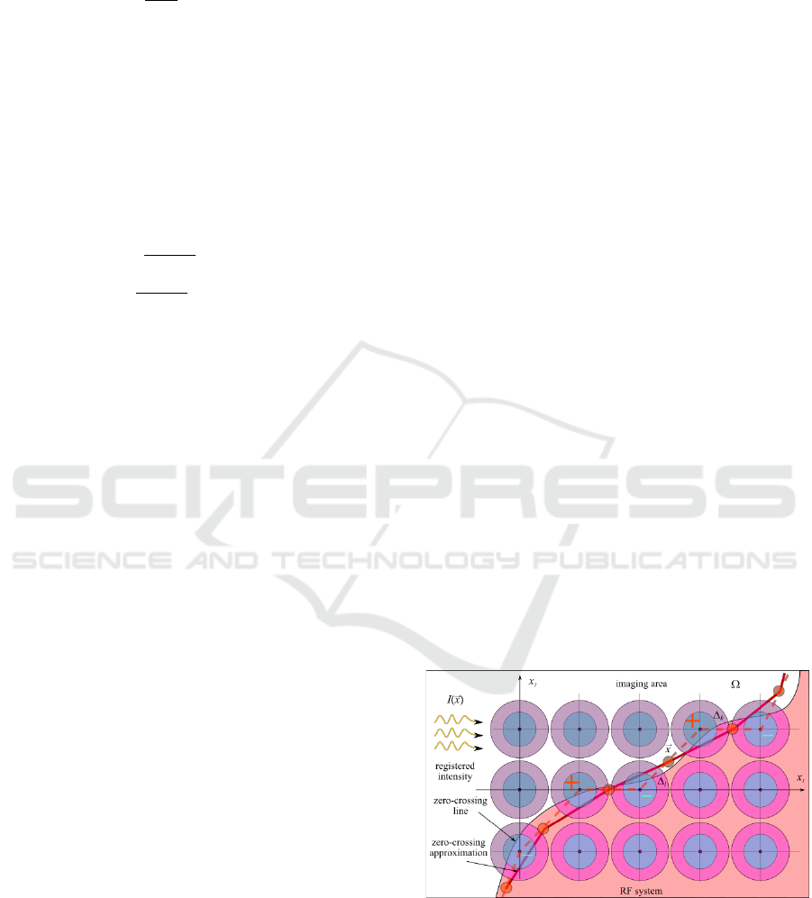
Figure 2: Marr's method for edge detection. The set of ON-
fields is marked with a “+” sign, the set of OFF-fields with
a “–” sign. Segments connecting the centres of the nearest
ON- and OFF-fields are marked with a dotted line. Zero-
points found by interpolation on these segments form a
broken line – zero-crossing approximation (edge).
ICPRAM 2024 - 13th International Conference on Pattern Recognition Applications and Methods
488

The first aspect is that, unlike the COSO filter
(Allebach, 1996), we cannot generate values of
at
arbitrary points of the image , but only at
locations
of a fixed discrete RF system
.
Therefore, the search for a solution to the nonlinear
equation
using standard, usually iterative,
methods encounter problems. Indeed, at some
iteration, the calculated approximation to the solution
may not coincide with one of the RF centres
,
which, due to the lack of data at such a point, will not
allow the search to continue. To solve this problem,
Marr proposed a method that models the work of
simple cells (neurons) located in the lateral geniculate
nucleus (Marr, 1980). The main idea of Marr is as
follows.
Let's consider a set of receptive fields with a
noticeable positive defect
and call them ON-
fields. Similarly, we call the set of fields that have a
negative defect
OFF-fields, see Figure 2.
Since these two sets do not intersect, they are
separated by some imaginary boundary. Any two
adjacent ON- and OFF-fields lying on both sides of
this boundary have defects of different signs,
therefore somewhere on the segment connecting them
there must exist a point at which
, as
shown in Figure 2. The position of this point can be
interpolated in any suitable way (for example, linear),
if the positions
and
of these fields and
corresponding values of their defects
and
are known. Having gone through all the pairs
of fields in this way and connecting the nearest points
found, we will obtain a broken zero-crossing line
approximation of the required zero-crossings as
shown in Figure 2.
The second aspect of the implementation is
related to the issues of reliably determining the
corresponding ON- and OFF-fields, i.e. with
questions of confident resolution of alternatives
. The problem here is that the recorded
defects
(6) are noisy data, which, with signal-
to-noise ratios , will often lead to false
decisions. The solution here is to use threshold
criteria of the type
or
with some threshold . However, this also raises
many questions like how to choose a threshold,
should it depend on the location
of the RF or on
the RF data
, etc. Some of the listed
issues for the case of Poisson counts were considered
in previous works, see for example, (Antsiperov,
2023). Below we discuss the adaptation of the
obtained results to current work.
3 IMAGE NEUROMORPHIC
ENCODING BY THE RF
SYSTEM
A statistical description of the image sampling
representation in the form of multivariate distribution
was obtained in
previous works (see for example (Antsiperov,
Kershner 2023) and looks as follows:
(10)
As has been shown, approximation (10) is valid
when sample size , where
is the average total number of counts registered
during exposure time at light intensity
.
Parameter
characterizes the interaction
of radiation with matter and depends on – the
average energy of the incident photon and on
dimensionless coefficient – the quantum efficiency
of detector material. It is noteworthy that distribution
(10) has several useful properties giving it a universal
character. (Antsiperov, Kershner 2023).
One of the important properties of (10) is that the
dependence of
on the intensity
is
almost trivial – it simply coincides with the value of
at the same point, up to the normalization
constant. This makes it possible to illustrate a typical
sampling representation, as well as its subsequent
processing results, using ordinary bitmap images and
considering their pixel values as an approximation of
the recorded intensity, expressed in some arbitrary
units.
Figure 3: Illustration of the image sampling representation.
On the left is the original, grayscale PNG image, on the
right is its representation
of the size
counts.
To illustrate a typical sampling representation for
a grayscale PNG image, we generated its
using the
Monte Carlo approach to sample from distribution of
Neuromorphic Encoding / Reconstruction of Images Represented by Poisson Counts
489

its pixels. An image and sampling representation are
shown in Figure 3. Grayscale PNG image is of size
pixels, color depth bits,
corresponding
is of size counts.
The generation of random counts was carried out by
using the Monte Carlo rejection/acceptance sampling
method with a uniform auxiliary distribution
and constant
.
It is easy to pass from a statistical description in
preset counts (10) to description in preset local
regions form (Barrett, 1997). Since the latter
description (preset regions) is more suitable for the
subsequent description of data associated with
receptive fields, we outline its brief conclusion here.
Namely, let's take some small region and
consider the event of a count into it as a success, and
the absence of count as a failure. According to (10),
the probability of success is
,
and of failure, respectively, . Then,
considering the registration of count as a test in the
Bernoulli scheme, we find that the probability of out
of successes – probability of counts of
in – is
determined by the binomial distribution, in
asymptotic , , but ,
coinciding with Poissonian:
(11)
where
is another parameter, however,
unlike depending also on the ratio of the sampling
representation
size to . For further purposes, it is
convenient to express the parameter of the Poisson
distribution (2) not through the registered intensity
, but through the intensity of counts generated by
receptors
, which is proportional to the first:
. Considering this notation, the
distribution of counts in (11) can be rewritten as
(12)
where is the area of region and
– the average
value of intensity of counts
per . Note that the
mean value of , as well as its dispersion according to
the Poisson distribution (12), is exactly
.
Let us use the notations introduced above for a
typical receptive field: – the RF region of the
area ,
– its centre / surround structure of
areas
respectively,
. Let us denote
the numbers of counts in the centre and in the
surround of RF by
and
. From the condition that
and
are the partition of it follows that
is the total number of counts on the RF. By
virtue of (12), the statistical models of
and
are
Poisson probability distributions:
(13)
where
and
are the average intensities of counts
in the centre and in the surround of RF:
(14)
Note here that since the numbers
and
are
unbiased estimates of their means
and
, the values
and
are unbiased
estimates of the average intensities
and
.
Since
and
are Poisson on the disjoint
regions
, they are statistically
independent, and their joint probability distribution
can be written as:
(15)
If we move from data
and
to random data
and
, then (15) turns into:
(16)
where
as well as (12) is the Poisson
probability distribution with the parameter
, and
is the binomial
distribution with parameters and
:
(17)
For a complete statistical description of the RF
data, it is necessary to select an a priori model of the
intensities
and
. In this regard, let us assume that
the marginal distributions of both intensities are given
by the same density . As for their joint
distribution, we will assume that two cases are
possible. In the first case, both intensities are
completely statistically dependent due to their
coincidence
, so their joint distribution is
, where is
Dirac delta-function. In the second case, they are
completely statistically independent, and their joint
distribution is
. Formally, denoting the
first case of complete dependence as the 0-hypothesis
, and the second one as its alternative
, we can
ICPRAM 2024 - 13th International Conference on Pattern Recognition Applications and Methods
490

write the a priori (conditional in relation to
) distribution of
and
in the form:
(18)
Combining (16) and (18), we obtain the following
distributions for the full statistical (generative) model
(19)
where due to
Δ
in the first line of the curly
brace in (19) the parameter
Δ
in
(17) is
replaced by
and the parameter in
(17) is replaced by
. In the second line of
the curly brace in (19) the original representation
(15) is used for
.
Marginalizing (19) we can find the unconditional
distribution
of random
and . After a
number of simplifications and approximations (see
(Antsiperov, 2023)), it can be approximated by the
following large-counts distribution:
(20)
Using (20), we can introduce the likelihood ratio
of the hypotheses
for given data
:
(21)
The likelihood ratio
(21) can be made
more interpretable by moving from the variables
to
and . For these variables
the binomial distribution admits a Gaussian
approximation (for large ). Also replacing
and
in (21)
by
, we get a simplified expression for the
likelihood ratio:
.
(22))
Basing on the likelihood ratio (22), one can use
the uniformly most powerful unbiased test (Young,
2005) to compare the degree of agreement between
hypotheses
to the available data . Namely,
according to the Neyman–Pearson criterion, one
should accept
– the hypothesis of the coincidence
, if
and reject
, implying
– the hypothesis of a significant difference
between
and
, otherwise. The threshold
clearly indicates its dependence on – the size of the
test. The test size, in its turn, can be defined as the
probability of falling into the critical region
, or
,
where
is given by the first line of the
curly brace (20). Having performed all the
summations (integrations), one can arrive at the
following explicit form of the the critical region
:
.
(23))
The right side of (23) can be simplified if we
approximate a priori distribution
by the value
on its characteristic scale . As the a priori
average of the number of counts on the RF is
approximately , we can replace
by
and by in the right-hand side of (23). Thus
it will turn into a constant, which we denote by
:
.
(24))
From (23,24) the size of the test takes the form:
(25))
where it is taken into account that
and the standard complementary
error function is used. Relation (25)
implicitly relates and
and thus there is no need
to find the threshold
, when is given. In
accordance with (25),
can be calculated directly
from as an inverse error function
.
After
is fixed, the criterion for rejecting the
hypothesis
– the hypothesis of the coincidence
Δ
(i.e. accepting alternative
of intensity
jump of on RF) takes the following final form:
.
(26))
Returning to the original formulation of our
method for detecting edges using zero-crossing lines,
set out in the first section, we note the following here.
The unbiased estimates of the average intensities
,
(14) and
(16) can be given by the RF registered
data
,
and
. By definition of a
Neuromorphic Encoding / Reconstruction of Images Represented by Poisson Counts
491

random variable
specifies an
unbiased estimate of the value
. But, in view of
the proportionality
, we have relations
,
and
. Therefore, is an
unbiased estimate of
. Thus, zero-
crossing lines of
will also be zero-crossing lines
also of and the edge detection algorithm can
literally be reformulated in terms of the data
over all receptive fields. In this case, ON-fields are
determined by the positive condition on the right side
of (30), and OFF-fields by the negative. Moreover,
since the thresholds in these conditions depend on
, data
are also needed for all fields.
Finally, the formulation of the proposed edge
detection method in terms of RF data
,
has the form:
Step 1. For all receptive fields in positions
find,
basing on sampling representation
, the
numbers of counts
in the centres,
– in the
surrounds and
in the RF regions.
Using them, generate sufficient data
:
and
.
Step 2. Basing on the data
build the classes of
ON- and OFF-fields:
.
Step 3. For all pairs of nearest ON- and OFF-fields
find on the connecting their centres segments
, using
interpolation, zero-points
, see
Figure 2.
Step 4. Connect all found nearest zero points
with a broken line, thereby obtaining an
approximation of the desired zero-crossing line, see
Figure 2.
Note that in Step 2, not all the fields will be
classified as ON- or OFF-fields. Moreover, practice
shows that usually their number is noticeably less
than the number of all fields. This, by the way, gives
reason to call the method proposed an algorithm for
encoding a sample representation
, see in
this regard (Antsiperov, 2023). Moreover, if the
factor
in the test thresholds of Step 2 is of the
order of one, the tests can be reformulated as
and
, where the counts
difference
, and
represents centre-corrected estimates of the total
number of counts on the RF.
4 NEUROMORPHIC DECODING
(INTERPOLATION) OF RF
ENCODED DATA
To illustrate the capabilities of the method proposed,
we present below the results of image edge-directed
interpolation, based on the data
generated by
Figure 3 (right) sampling representation. To restore
(decoding) encoded images, the reconstruction area,
like the area of the original image , is covered with
a similar (in number, shape, and arrangement of
fields) RF system. For example, a RF system
consisting of 900 square fields, shown in Figure 4,
was used for encoding / restoration of the image and
its sampling representation, presented in Figure 3.
Figure 4: The result of RF encoding of image sampling
representation shown in Figure 3. On the left is a sampling
representation with a grid of 30×30 receptive fields, on the
right are RFs with a censored code
: white – ON-RFs with
, black– OFF-RFs with
.
Using this auxiliary RF system, a grid dual to it is
constructed, the nodes of which are the centres of the
corresponding RFs, and the edges are the segments
connecting the nearest nodes. To each -th node the
data (code)
of the -th RF is also assigned.
Classical bilinear image interpolation can be
constructed only from the “smooth” part of the code
. Namely, the
values are first interpolated
along the vertical edges of the grid, and then linearly
along all rows of all cells based on the already
interpolated vertical edges. The interpolation we
propose also uses two-pass reconstruction. During the
first pass, the
values are also interpolated along the
grid edges, not only vertical, but also horizontal.
What's important here is that this interpolation is not
necessarily linear. If at the nodes of a given edge the
values
and
are nonzero and have different signs,
then such an edge is considered as intersecting the
zero-crossing line – the line of contrast difference,
and the middle of the edge is taken as the intersection
(zero-) point. The interpolation in this case is
piecewise constant on both sides of this edge. In the
ICPRAM 2024 - 13th International Conference on Pattern Recognition Applications and Methods
492

second pass, the values in the grid cells are linearly
interpolated from the values on their edges.
Moreover, if a pair of cell edges intersects with the
zero-crossing line, then interpolation is carried out
along a segment connecting the zero-points. If not,
then interpolation is performed along the rows of
cells, as in classical interpolation. The results of both
types of interpolation are presented in Figure 5.
Figure 5: Interpolation based on the codes of Figure 4,
generated from the image of Figure 3. On the left – bilinear
interpolation of the image based only on the “smooth” part
of the code, on the right – interpolation of the image
along the zero-crossing line segments, specified also by the
“details”
.
5 CONCLUSIONS
A special feature of the proposed method is the
concept of receptive fields, widely used in its context.
The use of the RF structure allows one to effectively
overcome the known difficulties of numerical
algorithms that process mixtures with a large number
of components. This conclusion follows, among other
things, from the existing experience in computer
implementation of the method: all illustrative
materials presented in the work were obtained as part
of computational experiments. Experiments
confirmed the effectiveness of the method in terms of
memory resources / computation time. For example,
the encoding / reconstruction of 1000x1000 pixels, 8
bits colour depth image, presented in this work as an
illustration (see Figures 3, 4, 5), required a calculation
time of only a few milliseconds even in the case of
the densest grid of 150x150 nodes (22500
components).
In general, based on the results obtained, it seems
reasonable to express the hope that the approach
proposed in the work will find soon both further
theoretical development and fruitful use in applied
problems.
REFERENCES
Allebach, J., Wong, P.W. (1996). Edge-directed
interpolation. In Proceeding of the 3rd IEEE Int.
Conference on Image Processing, V. 2, P. 707–710.
doi: 10.1109/icip.1996.560768.
Antsiperov V. E. (2022). Generative Model of
Autoencoders Self-Learning on Images Represented by
Count Samples. In Automation and Remote Control. V.
83 (12), P. 1959-1983. doi: 10.1134/S00051179220120
098.
Antsiperov, V., Kershner, V. (2023). Retinotopic Image
Encoding by Samples of Counts. In Pattern
Recognition Applications and Methods. ICPRAM 2021
2022, De Marsico, M., Sanniti di Baja, G., Fred, A.
(eds). Lecture Notes in Computer Science, V. 13822.
Springer, Cham. doi: 10.1007/978-3-031-24538-1_3.
Antsiperov V. (2023) New Centre/Surround Retinex-like
Method for Low-Count Image Reconstruction. In
Proceedings of the 12th International Conference on
Pattern Recognition Applications and Methods
(ICPRAM 2023), SCITEPRESS – Science and
Technology Publications, Lda, P. 517-528. doi:
10.5220/0011792800003411.
Barrett, H., White, T., Parra, L. (1997). List-mode
likelihood. In J. Opt. Soc. Am. A, V. 14, P. 2914–2923.
doi:10.1364/JOSAA.14.002914.
Bear M. F., Connors B. W., Paradiso M. A. (2007). The eye.
In Neuroscience: Exploring the Brain, P. 277–307.
Christensen D. V., et al. (2022). 2022 roadmap on
neuromorphic computing and engineering. In
Neuromorphic Computing and Engineering. V. 2, P.
022501. doi: 10.1088/2634-4386/ac4a83.
Haralick, R. M. (1984). Digital Step Edges from Zero
Crossing of Second Directional Derivatives. In IEEE
Transactions on Pattern Analysis and Machine
Intelligence, PAMI-6(1), P. 58–68.
doi:10.1109/tpami.1984.4767475.
Kuffler S. W. (1953). Discharge patterns and functional
organization of mammalian retina. In Journal of
neurophysiology, V. 16(1), P. 37–68. doi:
10.1152/jn.1953.16.1.37
Land E. H. (1977). The Retinex theory of color vision. In
Scientific American, V. 237(6), P. 108–129. doi:
10.1038/scientificamerican1277-108
Marr, D., Hildreth, E. (1980) Theory of Edge Detection. In
Proceedings of the Royal Society of London. Series B,
Biological Sciences, V. 207(1167), P. 187–217.
Nguyen G., et al. (2019) Machine learning and deep
learning frameworks and libraries for large-scale data
mining: a survey. In Artificial Intelligence Review. V.
52, P. 77–124. doi: 10.1007/s10462-018-09679-z.
Young G. A., Smith R. L. (2005). Essentials of statistical
inference. Cambridge University Press. Cambridge.
Neuromorphic Encoding / Reconstruction of Images Represented by Poisson Counts
493
