Unsupervised Domain Adaptation for Human Pose Action Recognition

Mattias Billast

1 a

, Tom De Schepper

1,2 b

and Kevin Mets

3 c

University of Antwerp, Imec, IDLab, Department of Computer Science, Sint-Pietersvliet 7, 2000 Antwerp, Belgium

AI & Data Department, Imec, Leuven, Belgium

University of Antwerp Imec, IDLab, Faculty of Applied Engineering, Sint-Pietersvliet 7, 2000 Antwerp, Belgium

Keywords:

Domain Adaptation, Human Pose, GCN, Action Recognition.

Abstract:

Personalized human action recognition is important to give accurate feedback about motion patterns, but there

is likely no labeled data available to update the model in a supervised way. Unsupervised domain adaptation

can solve this problem by closing the gap between seen data and new unseen users. We test several domain

adaptation techniques and compare them with each other on this task. We show that all tested techniques

improve on the model without any domain adaptation and are only trained on labeled source data. We add

multiple improvements by designing a better feature representation tailored to the new user. These improve-

ments include added contrastive loss and varying the backbone encoder. We would need between 30% and

40% labeled data of the new user to get the same results.

1 INTRODUCTION

Human action recognition is essential to give per-

sonal feedback about body motions. It has appli-

cations in health, industry, and gaming (Pareek and

Thakkar, 2021). Examples are monitoring a user’s

health by their behavior, gesture recognition in gam-

ing, and faster and safer human-robot interactions.

Models are often trained on very large datasets but

we focus on new unseen subjects to immediately have

high-performant personalised models. Action recog-

nition on human pose data assigns action classes to a

sample of human pose frames. The performance of

the action recognition is strongly related to the data.

When testing on new subjects or new tasks, the per-

formance drops because of out-of-distribution sam-

ples. This can be because of the style of movement

of the new subject or because of different dimensions

and relations between joints. As labeling new data of

these new subjects is time-consuming and expensive,

unsupervised domain adaptation can offer a solution

to improve performance on these out-of-distribution

subjects or tasks. Figure 1 shows a simpliﬁed visual-

ization of the problem. In this paper, we test various

domain adaptation techniques with different combi-

nations of losses, backbones, and other hyperparame-

ters. We discuss the results from our experiments on

https://orcid.org/0000-0002-1080-6847

https://orcid.org/0000-0002-2969-3133

https://orcid.org/0000-0002-4812-4841

this topic and offer guidelines to tackle Domain adap-

tation on human action recognition. We used gen-

eral domain adaptation techniques as the literature is

limited for domain adaptation on human pose action

recognition. More advanced or newer domain adapta-

tion techniques are linked with the task and extract ad-

ditional performance from the data, goal, and model

architecture (Xu et al., 2022; Luo et al., 2020). This

paper could serve as a stepping stone for further re-

search on this topic.

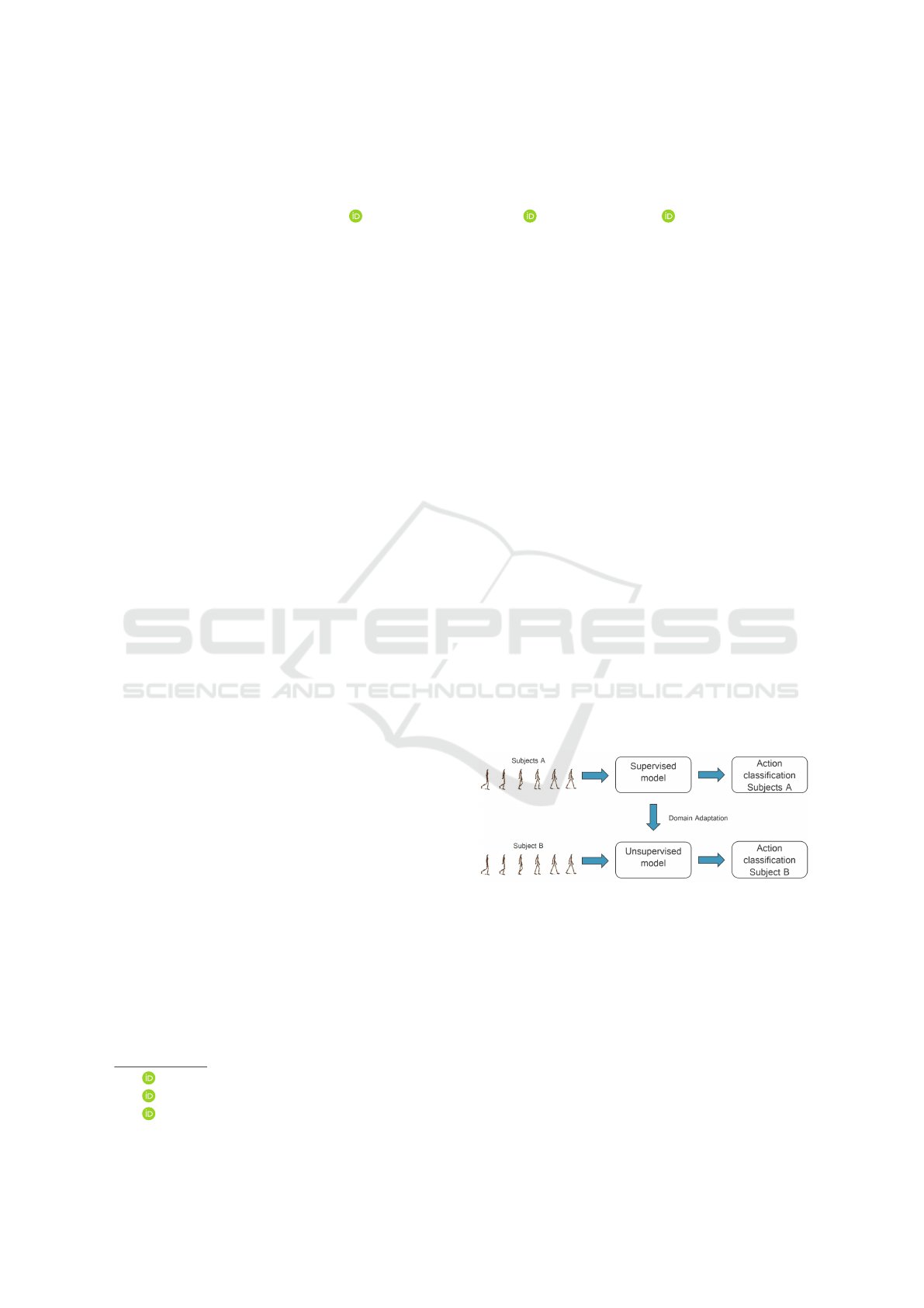
Figure 1: Simpliﬁed visualization of the problem. We adapt

a supervised action recognition model, trained on source la-

bels (subjects A), with domain adaptation techniques to per-

form better on unseen data from a target user (subject B).

The inputs for both models are human pose data.

2 RELATED WORK

For our related work, we focus on unsupervised do-

main adaptation and human pose action recognition.

Billast, M., De Schepper, T. and Mets, K.

Unsupervised Domain Adaptation for Human Pose Action Recognition.

DOI: 10.5220/0012573400003660

Paper published under CC license (CC BY-NC-ND 4.0)

In Proceedings of the 19th International Joint Conference on Computer Vision, Imaging and Computer Graphics Theory and Applications (VISIGRAPP 2024) - Volume 2: VISAPP, pages

837-844

ISBN: 978-989-758-679-8; ISSN: 2184-4321

837

2.1 Domain Adaptation

The main method to perform domain adaptation is

aligning both domains and creating discriminative

domain-invariant features. This can be done by metric

learning, adversarial learning, or data augmentation.

An example of metric learning is Maximum

Mean Discrepancy (MMD)(Long et al., 2013) by

matching the distributions of source and target do-

mains or Deep Reconstruction-Classiﬁcation Net-

work (DRCN) (Ghifary et al., 2016). Some exam-

ples of Adversarial techniques are Adversarial Bipar-

tite Graph Learning, which creates a domain-agnostic

video classiﬁer to overcome the limitations of adver-

sarial representation learning on videos (Luo et al.,

2020), Gradient Reversal Layer (GRL) (Ganin and

Lempitsky, 2015), Gradient Reversal Layer method

without the discriminator as the task-speciﬁc classi-

ﬁer is reused as a discriminator (Chen et al., 2022),

and Adversarial Discriminative Domain Adaptation

(ADDA) (Tzeng et al., 2017).

Domain adaptation can be done with data aug-

mentation of instances that bridge the gap between

source and target domains. A few examples are

Mixup (Zhang et al., 2017) which creates samples by

linearly interpolating between two instances of dif-

ferent domains, Vision Transformer utilizing Mixup

strategy exploiting cross-attention (Zhu et al., 2023)

to build an intermediate domain between source and

target, and Contrastive Vicinal Space (Na et al., 2022)

which alleviates the problem that the source labels are

dominant over the target labels by constraining the

model on vicinal instances to have different views and

labels in the contrastive space and agree in the consen-

sus space.

Other mechanisms to improve domain adaptation

are Cross-domain gradient discrepancy minimization

(Du et al., 2021) as it better represents the seman-

tic information, k-nearest neighbor classiﬁer after

feature fusion of multiple modalities (Lang et al.,

2019), cross-attention of transformers to create better

pseudo-labels of the target sample to improve the per-

formance(Xu et al., 2022), and generalization to tar-

get domain by including domain contrastive loss and

spatio-temporal contrastive loss on vision data (Song

et al., 2021).

2.2 Human Pose Action Recognition

There is limited related work on domain adaptation

for human pose action recognition. In (Tas and Ko-

niusz, 2018), they perform human action recognition

on 3D pose data by ﬁrst transforming the coordinate

data into a texture representation on which a CNN

(ResNet-50) is applied in combination with a domain

adaptation technique. Phase Randomization (Mit-

suzumi et al., 2024) disconnects the individuality and

action feature with self-supervised data augmentation

and data augmentation to randomize only the phase

component of the motion sequence. This creates a

subject-agnostic model.

3 DATASET

All our experiments are done on the H36M

Dataset (Ionescu et al., 2014). The dataset consists

of 6 subjects that performed 15 different actions. In

total, there are 3.6 million frames available within

the dataset with corresponding 3D human pose data.

The dataset has accurate 3D joint positions and joint

angles from a high-speed motion capture system at

50Hz. The kinematic tree of the human pose is com-

posed of 22 joints with XYZ coordinates relative to

the center of the hip joint. Before running the abso-

lute positions through a model, the data is normalized

between -1 and 1 in the three dimensions. Each frame

has an action ID ranging from 0 to 15.

The data split for testing is given by the same

frame numbers for each action and subject as in the

SRNN paper (Jain et al., 2016). The training split is

given by frame numbers such that there is no overlap

with the test data and that there is at least a two-frame

buffer to make sure there is no prior information about

the test data during training.

4 METHOD

Human action classiﬁcation takes T frames of human

poses with V joints as input and predicts the most

probable action class for that input. The goal is to

maximize the accuracy of the action classiﬁcation.

The domain adaptation setting in this paper assumes

the source domain with labeled data to be data from

subject(s) A and the target domain without labeled

data during the training phase of the model to be from

subject(s) B. The reason for this setup is to ﬁnd a per-

sonalized model that generalizes well to new out-of-

distribution data from new subjects.

The main goal of this paper is not to have the

highest performance of domain adaption but to see

which changes in architecture have the highest im-

pact. We did this by starting from a base model, adap-

tation technique, and hyperparameter tuning which

will serve as a reference baseline. By changing one

VISAPP 2024 - 19th International Conference on Computer Vision Theory and Applications

838

thing, we try to pinpoint the advantages or disadvan-

tages of certain changes to the model and setup.

4.1 Options

In this section, we list the various options of do-

main adaptation technique, backbone, and loss func-

tion from which we can choose variations to compare

with each other.

We tested four different Domain adaptation tech-

niques, i.e. Deep Reconstruction-Classiﬁcation Net-

work (DRCN) (Ghifary et al., 2016), Gradient Rever-

sal Layer (GRL) (Ganin and Lempitsky, 2015), Ad-

versarial Discriminative Domain Adaptation (ADDA)

(Tzeng et al., 2017), and Maximum Mean Discrep-

ancy (MMD)(Long et al., 2013). The ﬁrst three works

by adapting the feature representation of the target do-

main onto the source domain. The last one (MMD)

tries to match the distributions of the source and target

domain. We chose these techniques as they are gen-

erally applicable to each task, model, or data because

more advanced techniques extract additional perfor-

mance by making task-speciﬁc alterations.

We tested two backbones to compare different

strategies to extract structure from the data. As previ-

ously mentioned, we use a Graph convolutional net-

work with variable edge connections between nodes

in space and time. The other backbone we test is

a more standard convolutional neural network, i.e.

ResNet-50, which is designed to ﬁnd local structures

in the ﬁrst layers. There are enough examples where

they use a CNN on graph data (Ding et al., 2023)(Tas

and Koniusz, 2018). As the receptive ﬁeld increases

through the layers, a CNN can link joints separated

by more space and time.

As a last variation, we add Contrastive loss to cre-

ate clusters of the feature vectors per action in the

source domain. The reasoning behind this extra loss is

to also create more discriminative clusters per action

in the target domain when we map the target feature

space on the source feature space.

4.2 Baseline

To be more speciﬁc, we will now go over our choices

for the baseline model and explain the reasons for

each choice. For the backbone, we chose a Space-

Time-Separable Graph Convolutional Network (STS-

GCN)(Soﬁanos et al., 2021) as it is a natural way

to represent spatio-temporal relations of human pose

data and gather insights into the topic. It lowers the

number of parameters needed, compared to RNN or

CNN models, which is an advantage for real-time ap-

plications as it decreases inference speed. The train-

able adjacency matrices with full joint-joint and time-

time connections have attention properties as some

nodes/timeframes will be more important for the pre-

dicted action. For the domain adaptation technique,

we chose Adversarial Discriminative Domain Adap-

tation (ADDA) (Tzeng et al., 2017), as it is an unsu-

pervised domain adaptation technique that works with

any framework where a feature representation of the

input is available. The loss function for our baseline is

the cross-entropy loss function as it is the most com-

mon multi-class loss function. Other hyperparameters

like the learning rate, iterations of the discriminator,

and target encoder are optimized by iterating over a

range of possibilities for each hyperparameter.

4.3 Domain Adaptation

In this section, we explain all the used domain adap-

tation techniques in more detail.

4.3.1 ADDA

ADDA is a general unsupervised domain adaptation

technique and consists of three stages. First, an initial

classiﬁcation model, which is an encoder followed by

a classiﬁer, is trained on a large dataset of labeled

data sampled from the source domain. Then, a do-

main discriminator and target encoder, are trained al-

ternately. The input of the discriminator is the feature

vector from the source and target encoder, computed

by alternately encoding the source and target inputs.

After training, the discriminator should not be able to

distinguish the extracted feature encodings from the

source and target domain. This can be done by using

an inverted-label GAN loss, with the following loss

function for the domain discriminator:

disc

= −(1 −Y )log(1 − D(E(I))) −Y log(D(E(I)),

(1)

where Y represent the domain label, E(I) the encoded

feature from input I, and D(X) the prediction of the

domain classiﬁer with feature X as input. The dis-

criminator is trained by minimizing L

disc

, while the

encoder is trained by minimizing the cross-entropy

loss of the classiﬁer and maximizing L

disc

. Finally,

the target encoder is evaluated by feeding target sam-

ples which are mapped to an approximately domain-

invariant feature space and afterwards classiﬁed by

the source classiﬁer

4.3.2 GRL

Gradient Reversal Layer domain adaptation (Ganin

and Lempitsky, 2015) has similar components as

ADDA but only has 1 stage and everything is trained

Unsupervised Domain Adaptation for Human Pose Action Recognition

839

end-to-end. The encoder and classiﬁer are updated

with supervised training on source data by minimiz-

ing a Loss function L

. A domain discriminator uses

feature vectors from the encoder as input and out-

puts a domain label whether the input data is from

the source or target domain. The weights of the dis-

criminator are updated by minimizing a binary cross

entropy loss L

and the weights of the encoder θ

are updated by maximizing this loss L

. Maximiz-

ing the loss is accomplished by reversing the back-

propagation gradients between the encoder and the

discriminator. The gradients after the reversal layer

are −λ

∂L

∂θ

. This process incorporates target domain

information into the model without any labels.

4.3.3 MMD

Maximum Mean Discrepancy (Long et al., 2013) is

a domain adaptation method not based on individual

samples but by looking at the distribution of a group

of samples. Besides the supervised training on train-

ing data, the distributions of source and target data are

matched with the following formula of the empirical

estimate of MMD:

MMD

n(n − 1)

∑

i̸= j

k(x

, x

n(n − 1)

∑

i̸= j

k(y

, y

) −

∑

i, j

k(x

, y

) (2)

where n is the number of samples of data, x

is a

source data sample, y

is a target data sample, and k()

is a distance metric. In our case, we chose k() as a

Gaussian distance metric :

k(x

, y

) = exp(

−||x

− y

2σ

) (3)

4.3.4 DRCN

The Deep Reconstruction-Classiﬁcation Network

(DRCN) (Ghifary et al., 2016) is a domain adaptation

technique that is based on two mechanisms to train

a feature encoder. As with the other techniques, the

ﬁrst mechanism is the supervised training on source

data. The second mechanism is the unsupervised re-

construction of unlabeled target data. The ﬁrst part

makes sure the model can still classify the different

classes and the second part encodes information from

the target domain.

4.4 Backbone

In this section, we explain all the used backbones in

more detail.

4.4.1 STS-GCN

The STS-GCN (Soﬁanos et al., 2021) model con-

sists of Spatio-Temporal Graph Convolutional layers

(STGCN) followed by Temporal convolutional layers

(TCN). The STGCN layers allow full space-space and

time-time connectivity but limit space-time connec-

tivity by replacing a full adjacency matrix with the

multiplication of space and time adjacency matrices.

The obtained feature embedding of the graph layers is

decoded by four TCN layers which produce the fore-

casted human pose trajectories.

The motion trajectories in a typical GCN model

are encoded into a graph structure with VT nodes for

all body joints at each observed frame in time. The

edges of the graph are deﬁned by the adjacency matrix

∈ R

V T ×V T

in the spatial and temporal dimensions.

The information is propagated through the network

with the following equation:

(l+1)

= σ(A

st−(l)

(l)

) (4)

where H

(l)

∈ R

(l)

×V T

is the input to GCN layer l with

(l)

the size of the hidden dimension which is 3 for the

ﬁrst layer, W

(l)

∈ R

(l)

×C

(l+1)

are the trainable graph

convolutional weights of layer l, σ the activation func-

tion and A

st−(l)

is the adjacency matrix at layer l. The

STS-GCN model alters the GCN model by replacing

the adjacency matrix with the multiplication of T dis-

tinct spatial and V distinct temporal adjacency matri-

ces.

(l+1)

= σ(A

s−(l)

t−(l)

(l)

) (5)

where T different A

s−(l)

∈ R

V ×V

describe the joint-

joint relations for each of T timesteps and V differ-

ent A

t−(l)

∈ R

T ×T

describe the time-time relations for

each of V joints. This version limits the space-time

connections and reports good performance (Soﬁanos

et al., 2021). This matrix multiplication is practically

deﬁned as two Einstein summations.

t−(l)

vtq

nctv

= X

ncqv

(6)

s−(l)

tvw

nctv

= X

nctw

(7)

4.4.2 ResNet-50

The ResNet-50 model (He et al., 2015) is a deep con-

volutional network comprising 50 layers. The main

building blocks are convolutional layers and identity

blocks. The identity blocks take the input through

several convolutional layers and add the input with

the output again. This solved the problem of vanish-

ing gradients to be able to train larger models more

efﬁciently.

VISAPP 2024 - 19th International Conference on Computer Vision Theory and Applications

840

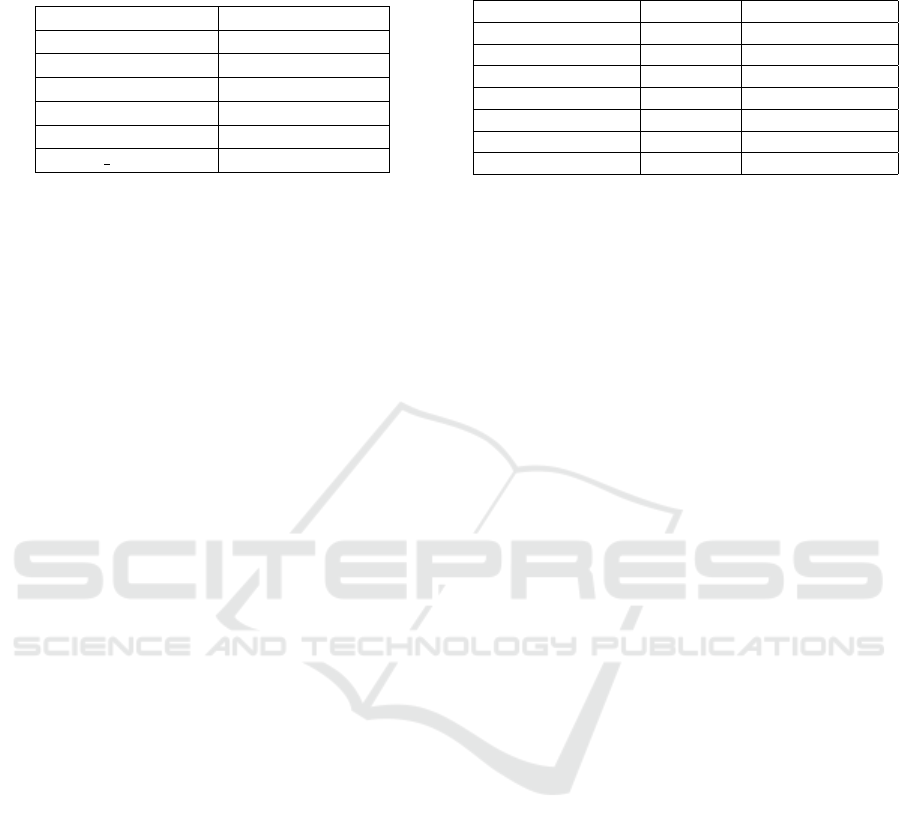
Table 1: Accuracy of different domain adaptation tech-

niques on the same baseline backbone and loss functions.

Domain Adaptation Average Accuracy

None 0.4470

ADDA 0.4941

MMD 0.4786

GRL 0.5012

DRCN 0.4669

DRCN t 0.4689

4.5 Contrastive Loss

Contrastive loss helps to discriminate better between

clusters. Speciﬁcally, it minimizes the distance be-

tween vectors from the same cluster and it maximizes

the distance between vectors from different clusters.

In our case, we used the Cosine similarity as a dis-

tance metric. The clusters are deﬁned by the action

classes and can only be used when training on source

data as we need the action labels for this contrastive

loss. But by increasing the discriminative power of

the source encoder, we hypothesize that the target en-

coder also improves when mapping target encodings

onto source encodings.

5 IMPLEMENTATION DETAILS

The GCN baseline model uses 4 TCN layers, and 4

STGCN layers (Soﬁanos et al., 2021). During train-

ing with ADDA, a range of learning rates were tested

and a learning rate of 1 × 10

−6

gave the best re-

sults for both updating the discriminator and target

encoder. The batch size is 256 for all experiments.

To update the weights, an Adam optimizer is used

with β

= 0.9, β

= −.999, and weight decay pa-

rameter λ = 1 × 10

−4

. The numbers of channels for

the STGCN layers are respectively 3, 64, 32, and 64,

and the number of channels for all four TCN layers is

equal to the output time frame. All models are trained

for 250 epochs with a learning rate scheduler which

lowers the learning rate by a factor γ = 0.2 when the

accuracy loss does not decrease for 10 steps. The

sampling of action classes is balanced based on the

number of occurrences in the dataset. To Train the

source encoder, the model is trained for 250 epochs

with a learning rate of 0.0005 and the same learning

rate scheduler as during the domain adaptation.

Table 2: Accuracy of different domain adaptation tech-

niques with different backbone.

Domain Adaptation Backbone Average Accuracy

S on T STS-GCN 0.4470

ADDA STS-GCN 0.4941

MMD STS-GCN 0.4786

GRL STS-GCN 0.5012

MMD ResNet-50 0.4959

GRL ResNet-50 0.5228

ADDA ResNet-50 0.5051

6 RESULTS

All accuracies shown in the tables are measured on

target data. The average accuracies are a combina-

tion of all accuracies where each subject is alternately

the target data and the source data is the remaining

subjects. We tested four different domain adaptation

techniques with the same backbone model and con-

ﬁgurations. As seen in Table 1, GRL has the best re-

sult on the baseline model, and DRCN the least. The

advantage of GRL is that it is end-to-end with mul-

tiple iterations over source and target data, whereas

ADDA needs more ﬁnetuning and has more poten-

tial suboptimal parameters during each training stage.

DRCN performs the worst as the reconstruction of

the input does not contain enough subject-agnostic

information to classify the action correctly. For the

reconstruction, the dimensions of the subject play a

more important role than the movement of the subject

which is essential to classify the action. To see the

inﬂuence of different backbones on the feature rep-

resentation, we experimented with a STS-GCN back-

bone and a ResNet-50 backbone. In Table 2, we see

that the ResNet50 model has an overall better perfor-

mance than the same model with a GCN backbone.

This means the CNN backbone can extract enough

structure from the input as the receptive ﬁeld is larger

than the input in our experiment. Shufﬂing the posi-

tion of the nodes decreases the performance as it takes

away the given structure of the kinematic tree, as the

nodes of the upper body, lower body, and limbs are

grouped initially. In Table 3 is shown that the CNN

backbone suffers the most in performance as it cannot

exploit local structures anymore. The GCN is robust

for different input variations. Table 4 shows that

2 STGCN layers is the optimal number of layers as

it avoids the over-smoothing effect of too many lay-

ers, i.e. more hops between nodes. With only one

layer, there is not enough information shared between

nodes. Added Contrastive loss adds performance in

combination with a ResNet-50 backbone as it cre-

ates more discriminative clusters in the feature space

Unsupervised Domain Adaptation for Human Pose Action Recognition

841

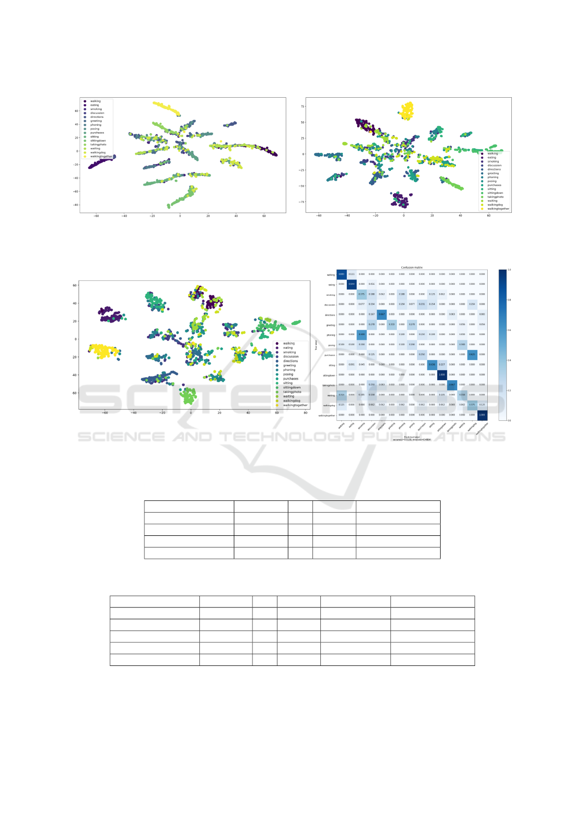
Figure 2: Visualization of the feature representation by T-SNE dimension reduction. On the left, is the feature representation

of the baseline model with ResNet-50 backbone and added CL loss, and on the right, is the same model but without CL loss.

Both representations are on target data from subject 9.

Figure 3: Visualization of the feature representation by T-SNE dimension reduction on the left and confusion matrix on the

right of the ResNet-50 model with GRL domain adaptation on subject 9 as target data.

Table 3: Accuracy of different domain adaptation techniques with different backbone and varying the input by shufﬂing the

order of the structured kinematic tree joints.

Domain Adaptation Backbone CL shufﬂed Average Accuracy

ADDA STS-GCN ✓ ✗ 0.4849

ADDA ResNet-50 ✓ ✗ 0.5002

ADDA STS-GCN ✓ ✓ 0.4756

ADDA ResNet-50 ✓ ✓ 0.4720

Table 4: Accuracy of different domain adaptation techniques with different backbones and varying the number of STGCN

layers in the backbone to create the feature representations.

Domain Adaptation Backbone CL shufﬂed STGCN layers Average Accuracy

ADDA STS-GCN ✓ ✗ 1 0.4800

ADDA STS-GCN ✓ ✗ 2 0.5003

ADDA STS-GCN ✓ ✗ 3 0.4893

ADDA STS-GCN ✓ ✗ 4 0.4849

ADDA STS-GCN ✓ ✗ 6 0.4892

VISAPP 2024 - 19th International Conference on Computer Vision Theory and Applications

842

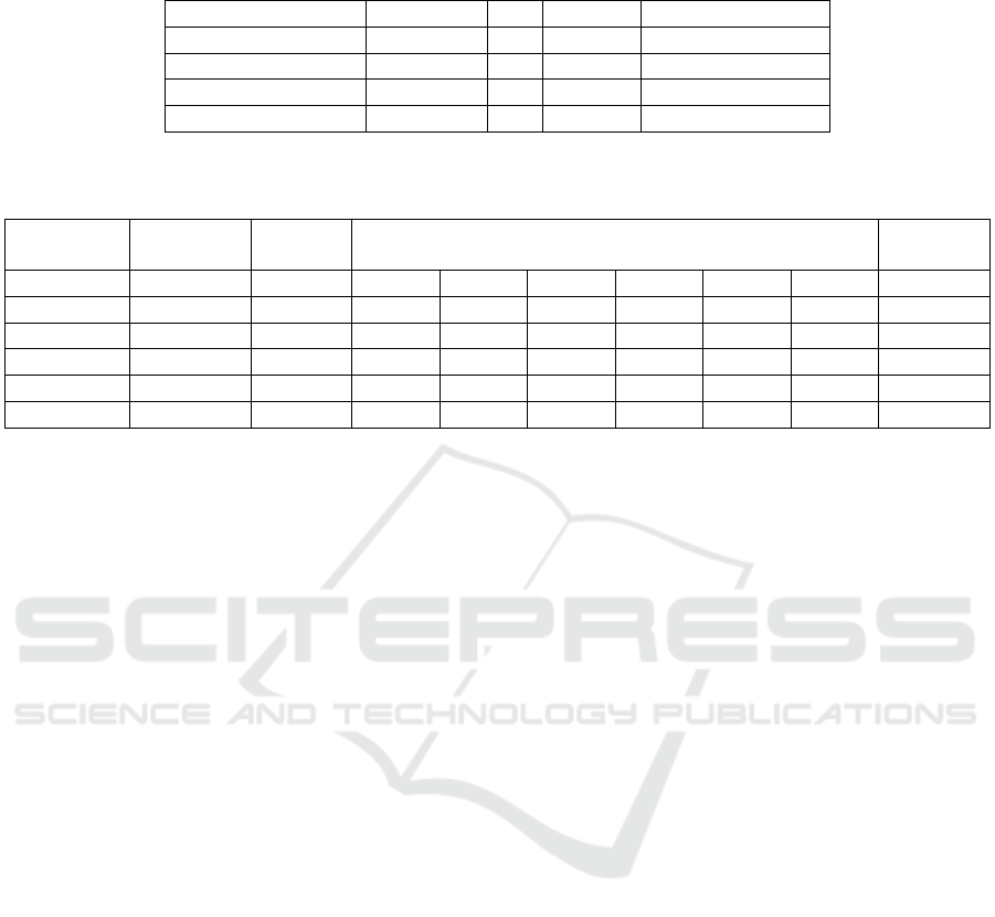
Table 5: Accuracy of different domain adaptation techniques with different backbone and adding a Contrastive Loss during

training on labeled source data.

Domain Adaptation Backbone CL shufﬂed Average Accuracy

ADDA STS-GCN ✗ ✗ 0.4941

ADDA ResNet-50 ✗ ✗ 0.5051

ADDA STS-GCN ✓ ✗ 0.5151

ADDA ResNet-50 ✓ ✗ 0.5002

Table 6: Detailed overview of accuracies per target subject of different models with various percentages of labeled target data

available during training compared with the best model with domain adaptation.

Domain Backbone % target Accuracy per target subject Average

Adaptation labels 9 8 7 6 5 1 Accuracy

None STS-GCN 0 0.4285 0.6437 0.3983 0.3258 0.4775 0.4084 0.4470

None STS-GCN 30 0.5393 0.5233 0.4747 0.4219 0.5046 0.3420 0.4676

GRL ResNet-50 0 0.5306 0.6437 0.4713 0.4546 0.5300 0.5067 0.5228

None STS-GCN 40 0.5554 0.6366 0.6126 0.4873 0.5853 0.4793 0.5594

None ResNet-50 100 0.9340 0.9627 0.9493 0.8846 0.9226 0.9313 0.9307

None STS-GCN 100 0.9379 0.9426 0.9473 0.8813 0.9400 0.9340 0.9305

which can be seen by the visualization of the features

by t-SNE dimension reduction, as can be seen in Fig-

ure 2. Table 5 shows that there is also a slight per-

formance increase when using an added contrastive

loss during pretraining on labeled source data. Table

6 shows that there is still a big gap between an Or-

acle (100% target labels) and the domain adaptation

models without any labeled target data. But when we

varied the number of target labels available, we con-

cluded that we needed between 30% and 40% of all

the available target labels to get the same result as the

best model with domain adaptation. Figure 3 shows a

visualization of the feature representation and confu-

sion matrix on one target subject for this best model

with domain adaptation.

7 DISCUSSION

In this paper, we test several domain adaptation tech-

niques on human pose motion data to classify actions.

The speciﬁc unsupervised domain adaptation in this

paper aimed to acquire personalized models for sub-

jects without any labeled information. We showed

that all these techniques improve the results on the

target data compared to the model only trained on la-

beled source data. We also varied the backbone and

concluded that a CNN can exploit the local structures

in the kinematic tree to improve the results. Con-

trastive Loss serves as an aid to improve the discrim-

inative power of the feature representations of the

source domain and consequently the target domain af-

ter domain adaptation. We need between 30% and

40% of target labels to close the gap between our best

domain adaptation model. This research serves as a

stepping stone for further research on domain adapta-

tion on human pose data. Possible extensions are fur-

ther expanding the number of adaptation techniques,

adding other data streams about the human pose like

rotational data, and testing on other datasets/classes.

ACKNOWLEDGEMENTS

This research received funding from the Flemish

Government under the “Onderzoeksprogramma Arti-

ﬁci

ele Intelligentie (AI) Vlaanderen” programme.

REFERENCES

Chen, L., Chen, H., Wei, Z., Jin, X., Tan, X., Jin, Y., and

Chen, E. (2022). Reusing the task-speciﬁc classiﬁer

as a discriminator: Discriminator-free adversarial do-

main adaptation. In Proceedings of the IEEE/CVF

Conference on Computer Vision and Pattern Recog-

nition (CVPR), pages 7181–7190.

Ding, X., Zhang, Y., Ge, Y., Zhao, S., Song, L., Yue, X.,

and Shan, Y. (2023). Unireplknet: A universal per-

ception large-kernel convnet for audio, video, point

cloud, time-series and image recognition.

Du, Z., Li, J., Su, H., Zhu, L., and Lu, K. (2021). Cross-

domain gradient discrepancy minimization for unsu-

pervised domain adaptation.

Ganin, Y. and Lempitsky, V. (2015). Unsupervised do-

main adaptation by backpropagation. In International

conference on machine learning, pages 1180–1189.

PMLR.

Ghifary, M., Kleijn, W. B., Zhang, M., Balduzzi, D., and

Li, W. (2016). Deep reconstruction-classiﬁcation

Unsupervised Domain Adaptation for Human Pose Action Recognition

843

networks for unsupervised domain adaptation. In

Computer Vision–ECCV 2016: 14th European Con-

ference, Amsterdam, The Netherlands, October 11–

14, 2016, Proceedings, Part IV 14, pages 597–613.

Springer.

He, K., Zhang, X., Ren, S., and Sun, J. (2015). Deep resid-

ual learning for image recognition.

Ionescu, C., Papava, D., Olaru, V., and Sminchisescu, C.

(2014). Human3.6m: Large scale datasets and pre-

dictive methods for 3d human sensing in natural envi-

ronments. IEEE Transactions on Pattern Analysis and

Machine Intelligence, 36(7):1325–1339.

Jain, A., Zamir, A. R., Savarese, S., and Saxena, A.

(2016). Structural-rnn: Deep learning on spatio-

temporal graphs.

Lang, Y., Wang, Q., Yang, Y., Hou, C., Huang, D., and Xi-

ang, W. (2019). Unsupervised domain adaptation for

micro-doppler human motion classiﬁcation via feature

fusion. IEEE Geoscience and Remote Sensing Letters,

16(3):392–396.

Long, M., Wang, J., Ding, G., Sun, J., and Yu, P. S. (2013).

Transfer feature learning with joint distribution adap-

tation. In Proceedings of the IEEE International Con-

ference on Computer Vision (ICCV).

Luo, Y., Huang, Z., Wang, Z., Zhang, Z., and Baktashmot-

lagh, M. (2020). Adversarial bipartite graph learning

for video domain adaptation. In Proceedings of the

28th ACM International Conference on Multimedia,

MM ’20. ACM.

Mitsuzumi, Y., Irie, G., Kimura, A., and Nakazawa, A.

(2024). Phase randomization: A data augmentation

for domain adaptation in human action recognition.

Pattern Recognition, 146:110051.

Na, J., Han, D., Chang, H. J., and Hwang, W. (2022). Con-

trastive vicinal space for unsupervised domain adap-

tation.

Pareek, P. and Thakkar, A. (2021). A survey on video-based

human action recognition: recent updates, datasets,

challenges, and applications. Artiﬁcial Intelligence

Review, 54:2259–2322.

Soﬁanos, T., Sampieri, A., Franco, L., and Galasso, F.

(2021). Space-time-separable graph convolutional

network for pose forecasting. In Proceedings of the

IEEE/CVF International Conference on Computer Vi-

sion (ICCV), pages 11209–11218.

Song, X., Zhao, S., Yang, J., Yue, H., Xu, P., Hu, R., and

Chai, H. (2021). Spatio-temporal contrastive domain

adaptation for action recognition. In Proceedings of

the IEEE/CVF Conference on Computer Vision and

Pattern Recognition, pages 9787–9795.

Tas, Y. and Koniusz, P. (2018). Cnn-based action recog-

nition and supervised domain adaptation on 3d body

skeletons via kernel feature maps.

Tzeng, E., Hoffman, J., Saenko, K., and Darrell, T. (2017).

Adversarial discriminative domain adaptation. In Pro-

ceedings of the IEEE conference on computer vision

and pattern recognition, pages 7167–7176.

Xu, T., Chen, W., Wang, P., Wang, F., Li, H., and Jin, R.

(2022). Cdtrans: Cross-domain transformer for unsu-

pervised domain adaptation.

Zhang, H., Ciss

e, M., Dauphin, Y. N., and Lopez-Paz, D.

(2017). mixup: Beyond empirical risk minimization.

CoRR, abs/1710.09412.

Zhu, J., Bai, H., and Wang, L. (2023). Patch-mix trans-

former for unsupervised domain adaptation: A game

perspective.

VISAPP 2024 - 19th International Conference on Computer Vision Theory and Applications

844