Numerical Modelling and Simulation of a Lab-on-a-Chip for Blood

Cells’ Optical Analysis

Ahmed Fadlelmoula

1,2

, Vítor Carvalho

3,4

, Susana O. Catarino

1,2

and Graça Minas

1,2

Center for MicroElectromechanical Systems (CMEMS-UMinho), University of Minho, 4800-058 Guimaraes, Portugal

LABBELS–Associate Laboratory, Braga/Guimaraes, Portugal

2Ai, School of Technology, IPCA, 4750-810 Barcelos, Portugal

Algoritmi Research Center, University of Minho, 4800-058 Guimaraes, Portugal

Keywords: Lab-on-a-Chip, Microfluidics, Numerical Simulation, COMSOL Multiphysics.

Abstract: Blood is a treasure of information about the functioning of the whole body. Thus, there is a continuous need

for new, accurate, fast, and precise techniques to analyse blood samples. The goal of this work is to design

and numerically simulate a low-cost lab-on-a-chip device, which, in the future, can be used to quickly

diagnose diseases by using a tiny drop of a blood sample from the patient. The designed microdevice includes

two fluid inlets, a serpentine area for achieving a continuous and fully developed flow, as well as a detection

chamber able for optical measurements. The numerical model of the designed microdevice was computed

using COMSOL Multiphysics software, taking into account the flow and tracking of microparticles,

mimicking blood cells. In order to reach the best lab-on-a-chip geometry, i.e., achieving a high and stable

number of particles in the detection chamber during the entire microfluidic assay, the inlet velocity, the

channel width, and the diameter of the detection chamber were individually optimized. A mesh study was

also performed to achieve the best results’ accuracy, with lowest computational effort. From the achieved

results, it was observed that a lab-on-a-chip geometry with a 0.5 mm channel width and a 2- or 3-mm detection

chamber radius, with a fluid inlet velocity of 3 mm/s, was the one with the most interesting results for the

intended application, with a constant number of particles flowing through the detection chamber (142 in

average, for the selected inlet conditions).

1 INTRODUCTION

Blood is a treasure of information about the

functioning of the whole body. Every minute, the

entire blood volume circulates throughout the body,

delivering oxygen and nutrients to every cell and

transporting products from and toward all different

tissues. As a result, blood harbors a massive amount

of information about the functioning of all tissues and

organs in the body Kouzehkanan et al., 2022).

Consequently, blood sampling and analysis are of

prime interest for medical and science applications

and hold a central role in diagnosing several

physiologic and pathologic conditions, localized or

systemic. However, for clinical and scientific

applications, it is necessary to understand, not only

the biology, but also the technologies involved

(Balogh, 2016). The knowledge about blood has

always evolved in parallel with the general

knowledge of biology, and several breakthroughs

were facilitated by technological advances. More

specifically, numerous devices are used to analyze

blood cells with good sensitivity. Various techniques

have been used for detecting platelets, white and red

blood cells (Rohde, 2015), with a continuous need

for fast, and precise techniques for the blood samples

analysis. Microfluidics has demonstrated an

enormous potential in this field. However, designing

a customized microfluidic platform, and gaining a

better understanding of its operation and the

underlying physics and mechanics still pose

significant technical challenges. On one hand,

experimental approaches, although expensive and

laborious, have been commonly used for the

development of microfluidic devices since they are

accurate and evidence-based methods (Fadlelmoula,

2022). Numerical approaches, on the other hand, are

now recognized as a reliable complementary method

aiming a reduction of cost, time, and effort, while

being relatively accurate (Nagarajan, 2017). So, this

Fadlelmoula, A., Carvalho, V., Catarino, S. and Minas, G.

Numerical Modelling and Simulation of a Lab-on-a-Chip for Blood Cells’ Optical Analysis.

DOI: 10.5220/0012571900003657

Paper published under CC license (CC BY-NC-ND 4.0)

In Proceedings of the 17th International Joint Conference on Biomedical Engineering Systems and Technologies (BIOSTEC 2024) - Volume 1, pages 185-190

ISBN: 978-989-758-688-0; ISSN: 2184-4305

185

work aims to design, simulate and optimize a low-

cost lab-on-a-chip (LOC) device, which can be used

to quickly evaluate and analyze blood cells using

optical methods. It presents the numerical modelling

and the simulation study of an optimized

microchannel geometry for the intended application.

Therefore, it simulates the flow of a buffer fluid

(representing plasma) filled with microparticles,

mimicking flowing blood cells. The microdevice will

comprise a serpentine region, for achieving a fully

developed flow (Catarino, 2019), as well as a

detection chamber, where the optical measurements

will occur, where the number of particles/cells should

be as high and steady as possible during the entire

duration of the assays.

This paper is organized into 5 sections: Section 2

presents the numerical methods; Section 3 shows the

obtained results; Section 4 presents the discussion;

and Section 5 enunciates the conclusions and further

developments.

2 NUMERICAL METHODS

This section describes the numerical simulation

methods applied for simulating the designed

microdevice.

2.1 2D Geometry Model

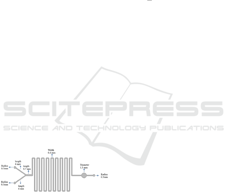
Figure 1 shows the initial lab-on-a-chip design

geometry. According to the computational results

(section 3), it will be optimized.

Figure 1: LOC initial design.

As can be observed in Figure 1, the total chip

dimension, 2D top view, is 4 cm length and 1.6 cm

width, there are 2 inlets and an outlet with a 0.5 mm

radius. The serpentine turn width is 0.4 mm, and the

circular detection chamber has a 1.3 mm diameter.

Relatively to the domains’ materials and properties,

the microchannel walls are constituted by

polydimethylsiloxane (PDMS) while, in the interior

of the device, water (1000 kg/m³ density and 0.001

Pa·s viscosity) will be flowing (Norouzi, 2017).

2.2 Governing Equations

The COMSOL Multiphysics Laminar Flow interface

(COMSOL, 2017) is used to compute the velocity and

pressure fields for the flow of a single-phase fluid in

the laminar flow regime. Equations (1) and (2)

present the fluid flow governing equations:

𝜌







𝑢∗∇𝑢



∇𝑃∇.𝜏 (1)

𝜏𝜂



𝛻𝑢  𝛻𝑢





2𝜂 𝐷 (2)

Where ρ represents the density,

∇

represents the

gradient operator, u is the velocity vector, t is time, P

is pressure, τ represents the Newtonian extra stress

tensor, η is the dynamic viscosity, T is the matrix

transpose, and D is the Symmetric rate of strain

tensor.

Besides the laminar flow, particle tracing for the

fluid flow was used as a numerical method for

computing the paths and migration of individual

particles by solving their equations of motion over

time. The particle traceability will be examined under

different conditions, to reach the maximum number

of particles that will pass through the detection

chamber. Equation (3) presents the particle tracing

governing equation:

𝐹𝑡  𝑑



𝑚𝑝𝑣



/𝑑𝑡

(3)

where Ft, mp, and v are, respectively, the total

force, the particle mass, and the particle velocity.

Particles moving through a fluid are subjected to a

force, known as drag force, which acts in the direction

of the fluid’s motion relative to the object. Equation

(4) presents the Stokes’ law equation, that allows to

determine the drag force (FD).

𝐹𝐷  6π ∗ 𝜇 ∗ 𝑟𝑝 ∗ 𝑢𝑠 (4)

where rp is the radius of the sphere and us is the

velocity of the fluid relative to the sphere, also called

slip velocity.

2.3 Boundary and Initial Conditions

The following boundary and initial conditions were

considered:

Laminar Flow: The default boundary condition in

laminar flow is a non-slip wall, which means that the

fluid velocity at the wall is zero.

Two different inlets were considered in the

microchannel, one for the particle’s inlet and other for

the buffer solution (Inlet 1 and Inlet 2). Both of them

are independently described by fluid velocities, that

range from 1 to 8 mm/s. At the outlet, a zero pressure

BIODEVICES 2024 - 17th International Conference on Biomedical Electronics and Devices

186

boundary is set to assure the outflow. Regarding the

numerical initial conditions, both initial velocity and

pressure were set to zero.

Particle Tracing for Fluid Flow: The boundary

condition in particle tracing was assumed as a

slipping particle wall, which means particles reflect

from the wall, such that the particle momentum is

conserved.

Regarding the inlet of particles, these were

released on both inlets, since the beginning of the

assay (time = 0 s), and at time steps of 0.1 seconds,

for a total duration of 15 seconds. At each 0.1 second

release, 200 rigid, non-charged particles (as an

approximation to flowing cells), entered the

microchannel. The number of particles was selected,

aiming to represent the number of blood cells in a

diluted whole blood sample, flowing in the channel.

In these simulations, the particles have a 5 μm

diameter and a 1050 kg/m³ density, representing the

size and density of red blood cells.

2.4 Mesh

After defining the numerical model, the geometry was

meshed, aiming its computational solution. To reach

the best type of mesh, aiming the most accurate

results with lowest computational cost, a mesh study

was performed. For that, simulations of the fluid flow

were performed in three different regions of the

microdevice, and the maximum fluid velocity

was evaluated in each of those regions, as shown in

Figure 2.

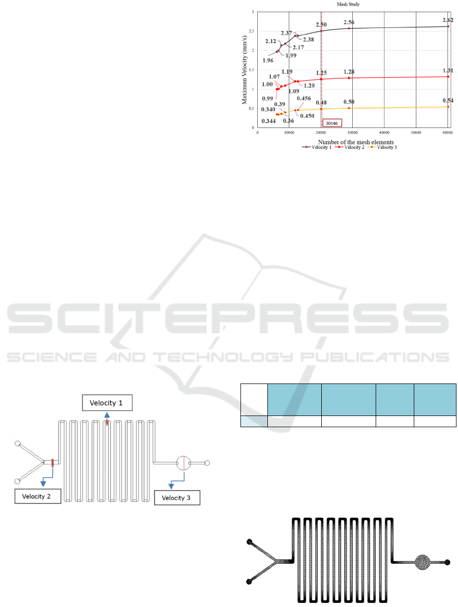
Figure 2: Schematic of the three regions where the

maximum velocity was evaluated during the mesh study

simulations.

After computing the model for 9 different meshes

(predefined at COMSOL Multiphysics), the

maximum velocity was evaluated in each of the 3

sections. Figure 3 shows the maximum velocity, at

each of the three regions (Velocity 1, Velocity 2 and

Velocity 3), for all the simulated meshes.

Figure 3: Maximum velocity (mm/s) in the microchannel as

a function of the number of mesh elements.

From the presented plot, it can be observed that,

above the 20146 elements mesh (“Finer” mesh, in

COMSOL), even if the number of elements is

increased (obviously with higher computational

efforts, since the number of calculus points’ increases

significantly), there is no significant variation or

improvement in the maximum velocity in any of the

considered regions. As it reaches a plateau, it will be

considered as the ideal mesh for this model, as it

allowed to achieve accurate results, without an

excessive computational cost (both regarding time

and memory). Thus, the statistics of the selected

“Finer” mesh, as predefined in COMSOL

Multiphysics, are shown in table 1.

Table 1: Mesh Statistics.

Minimum

Element

Qualit

Average

Element

Qualit

Mesh

Vertices

Triangles

Fine

0.5016 0.8256 9351 20146

This mesh, with 20146 triangular elements (9351 of

them mesh vertices), achieved the best results in

terms of velocity stability and computational time.

This mesh has a minimum element quality of 0.5016

(0-1 scale) and an average element quality of 0.8256,

and it is represented in figure 4.

Figure 4: Representation of the 2D finer mesh.

Numerical Modelling and Simulation of a Lab-on-a-Chip for Blood Cells’ Optical Analysis

187

2.5 Solver

The laminar flow, as a steady-state condition, was

simulated using a stationary solver. The particle

tracing was simulated considering a time-dependent

solver, for a total duration of 15 seconds, with 0.1 s

time steps.

3 RESULTS AND DISCUSSION

The simulated results, using COMSOL Multiphysics,

were achieved considering the effect of the fluid flow

(velocity and pressure profile along the lab-on-a-chip)

and of the particle’s migration in the detection

chamber. For achieving a high and stable number of

particles in the detection chamber during the entire

microfluidic assay, the inlet velocity, the channel

width, and the diameter of the detection chamber

were individually optimized, outputting the best LOC

geometry.

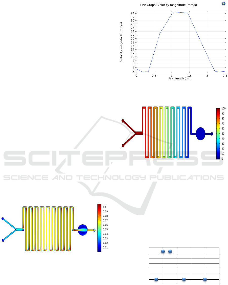
With the layout geometry described in Figure 1,

Figure 5 shows the plot of the fluids’ velocity

magnitude during the migration along the

microdevice. Analyzing Figure 6, that represents the

velocity profile through a half-width cut of one of the

simulated detection chambers, it can be concluded

that the velocity in the near wall region decreases,

being 0 at the wall, and being maximum at the center

of the detection chamber. Moreover, figure 7 shows

that the obtained pressure varies along the LOC

channels from the highest at the beginning of the

microdevice, decreasing gradually until the end of the

microdevice.

Figure 5: Stationary velocity magnitude (mm/s) in the

microdevice.

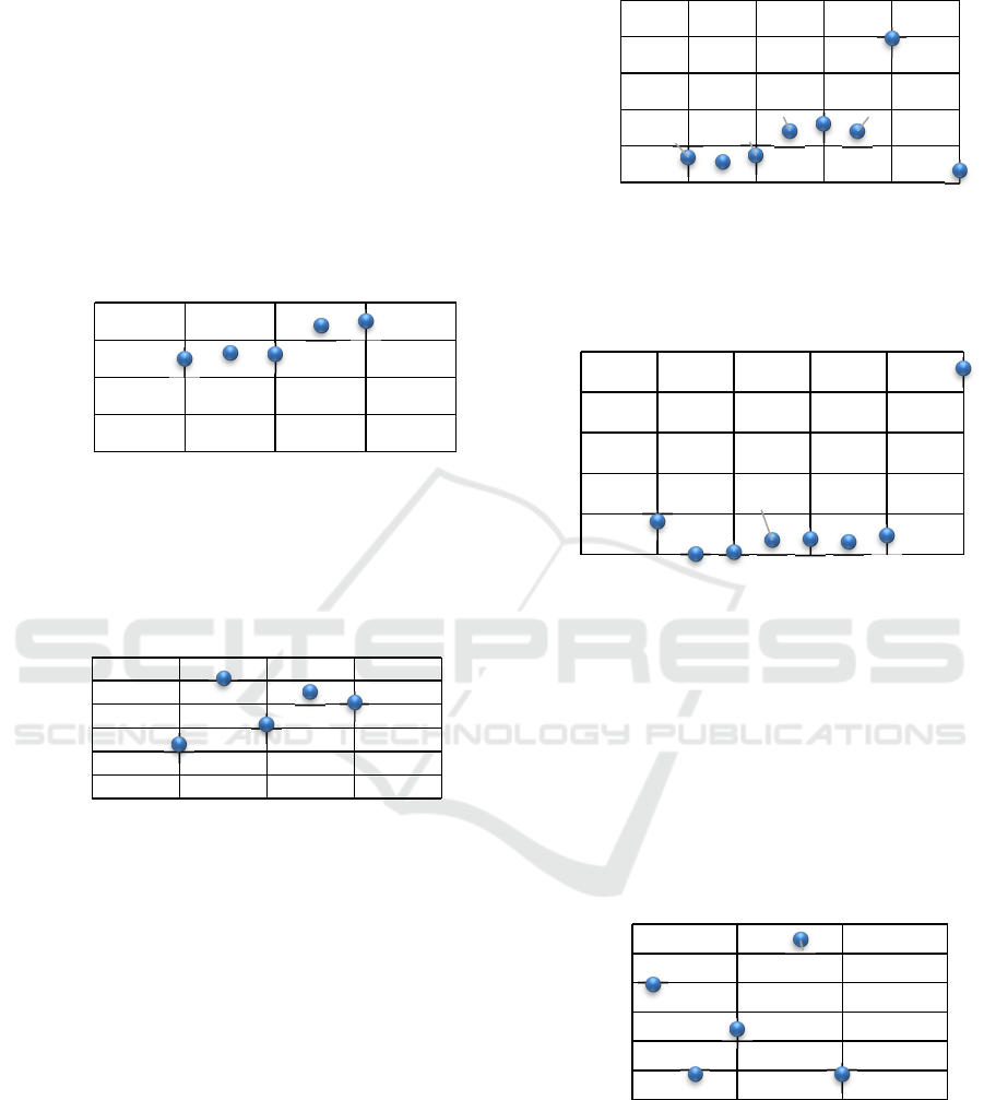
The first layout geometry optimization was

performed fixing the channel width and the detection

chamber radius, and changing the inlet velocity. The

channels' width was kept at 0.4 mm and the detection

chamber radius as 1 mm. The velocity was changed

being 1, 2, 3, 5 and 8 mm/s. Figures 8 show the

average of the number of particles that passed through

Figure 6: Example of a cross-section plot of the stationary

velocity magnitude (mm/s), at the detection chamber half-

width.

Figure 7: Pressure distribution along the microdevice.

the detection chamber, respectively, during the entire

duration of the experiment (15 seconds). The results

show that modifying the inlet velocity, from 1 to 8

mm/s, has no significant effect in the number of

particles crossing the detection chamber (it was

always around 25 particles at any time). As the 2

mm/s and 3 mm/s inlet velocities reached the exact

same average results, a 3 mm/s inlet velocity was

selected for the next optimization steps due to their

slightly higher particles number passing through the

detection chamber.

Figure 8: Average number of particles that passed through

the detection chamber, for different inlet velocities.

25.05

25 25

24,99

25,01

25,02

25,03

25,04

25,05

25,06

0246810

Average number of

particles (a.u.)

Particles velocity at inlet (mm/s)

BIODEVICES 2024 - 17th International Conference on Biomedical Electronics and Devices

188

In the second experiment, the channel width (0.4 mm)

and the inlet velocity (3 mm/s) were fixed, and the

detection chamber radius was changed from 1 to 3

mm in steps of 0.5 mm. Figures 9 and 10 show the

average and standard deviation of the number of

particles that passed through the detection chamber,

respectively, during the duration of the simulation (15

seconds). The results show that, increasing the radius

of the detection chamber leads to an increase of the

average number of particles in that area. Thus, a 3 mm

radius (with an average number of particles around

35) was selected for the next optimization steps.

Figure 9: Average number of particles that passed through

the detection chamber, for different detection chamber

radius.

Figure 10: Standard deviation of the number of particles

passing through the detection chamber, for different

detection chamber radius.

In the third experiment, the inlet velocity (3 mm/s)

and the detection chamber radius (3 mm) were fixed

and the width of the channels was varied from 0.2 to

1 mm in steps of 0.1 mm. Figures 11 and 12 show the

average and standard deviation of the number of

particles that passed through the detection chamber

during the duration of the assay (15 seconds),

respectively. From the average and the standard

deviation obtained results, an adequate channel width,

combining a high and stable number of particles in the

chamber is 0.5 mm.

Figure 13 shows the number of particles that passed

through the detection chamber when changing the inlet

2 velocity and maintaining the previously optimized

detection chamber radius (3 mm), channel width

Figure 11: Average number of particles that passed the

detection chamber, for different channels’ width.

Figure 12: Standard deviation of the number of particles

passing through the detection chamber, for different

detection channels width.

(0.5mm) and inlet 1 velocity (3 mm/s). It was verified

that no significant changes occurred regarding the

particle number that passed in the detection chamber.

This means that, for the studied geometries and inlet

conditions, the change in the inlet 2 velocity (buffer)

will not change the particle number.

Figure 13: Average number of particles that passed the

detection chamber, for different inlet 2 velocities.

From the results presented in the previous plots,

Figure 14 shows the instantaneous number of

particles passing through the detection chamber when

a 0.5 mm channel width, a detection chamber radius

25.05

26.42

26.10

33.73

35.05

01234

Average number of

particles (a.u.)

Detection chamber radius (mm)

0.22

0.50

0.31

0.45

0.40

0,1

0,2

0,3

0,4

0,5

0,6

01234

Standard deviation

(a.u.)

Detection chamber radius (mm)

69.28

73.05

141.58

159

141

395.58

33.33

100

200

300

400

500

0 0,2 0,4 0,6 0,8 1

Average number of

particles (a.u.)

Channels width (mm)

3.24

0.22

1.37

1.52

1.19

1.85

18.38

0 0,2 0,4 0,6 0,8 1

Standard deviation (a.u.)

Channels width (mm)

94.84

94.69

94.76

94.92

94.69

94,65

94,7

94,75

94,8

94,85

94,9

94,95

0 5 10 15

Average number of

particles (a.u.)

Inlet 2 velocity

Numerical Modelling and Simulation of a Lab-on-a-Chip for Blood Cells’ Optical Analysis

189

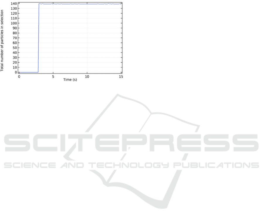
of 3 mm and an inlet velocity of 3 mm/s was

considered. It can be observed that, after the particles

first reach the detection chamber (shortly before 6

seconds), the number of particles keeps stable and

almost constant during the assays.

Figure 14: Total number of particles passing in the detection

chamber over each time instant, considering the optimized

design.

4 CONCLUSION AND FUTURE

WORK

This works presented the design and numerically

simulation of a LOC device with optimized

dimensions, regarding inlets velocities, channel

width, and diameter of the detection chamber for

achieving a high and stable number of particles in the

detection chamber. The numerical model was

computed, using COMSOL Multiphysics software,

taking into account the flow and microparticles

tracking, mimicking the blood cells.

The obtained results showed the ideal design, a 0.5

mm channel width, a detection chamber radius of 2

mm or 3 mm, and an inlet velocity of 3 mm/s,

achieving a total number of 142 particles flowing in

the detection chamber (see figure 11). The change of

the channels width made the major difference, when

compared with the others changed parameters, in the

number of particles passing through the detection

chamber. Regarding the flow, the pressure along the

LOC reached the maximum value at the inlet and

decreased gradually until reached the minimum in the

outlet. The stationary velocity reached the maximum

value in the serpentine channels and at the center of

the detection chamber.

Further work will consolidate the physical

implementation of the simulated LOC model and

their testing, examining the velocity, pressure, and

particle flow inside the chip, and performing design

updates if required.

ACKNOWLEDGMENTS

This work was supported by the R&D Unit Project

Scope: UIDB/04436/2020, UIDB/05549/2020 and

UIDP/05549/2020 funded by the Foundation for

Science and Technology, I.P. (FCT). A.F. thanks the

FCT for his 2023.03312.BD PhD grant. S.O.C. thanks

the FCT for her 2020. 00215.CEECIND contract

funding (DOI: 10.54499/2020.00215.CEECIND/

CP1600/CT0009).

REFERENCES

Balogh, E. P., Miller, B. T., & Ball, J. R. (2016). Improving

diagnosis in health care. In Improving Diagnosis in

Health Care. National Academies Press. https://doi.org/

10.17226/21794

Catarino, S. O., Rodrigues, R. O., Pinho, D., Miranda, J. M.,

Minas, G., & Lima, R. (2019). Blood cells separation

and sorting techniques of passive microfluidic devices:

From fabrication to applications. In Micromachines

(Vol. 10, Issue 9). MDPI AG. https://doi.org/10.3390/

mi10090593

COMSOL Multiphysics User’s Guide. 2017. Available

online: doc.comsol.com/5.4/doc/com.comsol.help.com

sol/COMSOL_ReferenceManual.pdf (accessed on 1

September 2023).

Fadlelmoula, A., Pinho, D., Carvalho, V. H., Catarino, S. O.,

& Minas, G. (2022). Fourier Transform Infrared (FTIR)

Spectroscopy to Analyse Human Blood over the Last 20

Years: A Review towards Lab-on-a-Chip Devices. In

Micromachines (Vol. 13, Issue 2). MDPI.

https://doi.org/10.3390/mi13020187.

Kouzehkanan, Z. M., Saghari, S., Tavakoli, S., Rostami, P.,

Abaszadeh, M., Mirzadeh, F., Satlsar, E. S.,

Gheidishahran, M., Gorgi, F., Mohammadi, S., &

Hosseini, R. (2022). A large dataset of white blood cells

containing cell locations and types, along with

segmented nuclei and cytoplasm. Scientific Reports,

12(1). https://doi.org/10.1038/s41598-021-04426-x

Nagarajan, S., Stella, L., Lawton, L. A., Irvine, J. T. S., &

Robertson, P. K. J. (2017). Mixing regime simulation and

cellulose particle tracing in a stacked frame

photocatalytic reactor. Chemical Engineering Journal,

313, 301–308. https://doi.org/10.1016/j.cej.2016.12. 016.

Norouzi, N., Bhakta, H. C., & Grover, W. H. (2017). Sorting

(Multiphysics®)cells by their density. PLoS ONE,

12(7). https://doi.org/10.1371/journal.pone.0180520

Rohde, T., & Martinez, R. (2015). Equipment and Energy

Usage in a Large Teaching Hospital in Norway. In

Journal of Healthcare Engineering · (Vol. 6, Issue 3).

BIODEVICES 2024 - 17th International Conference on Biomedical Electronics and Devices

190