Automatic Computation of the Posterior Nipple Line from

Mammographies

Quynh Nhu Jennifer Tran

, Tina Santner

2 a

and Antonio Rodr

ıguez-S

anchez

1 b

Department of Computer Science, University of Innsbruck, Innsbruck, Austria

Department of Radiology, Medical University of Innsbruck, Innsbruck, Austria

Keywords:

Mammogram, Posterior Nipple Line Detection, Computer Vision.

Abstract:

Breast cancer is the most commonly diagnosed cancer in female patients. Detecting early signs of malignity

by undergoing breast screening is therefore of great importance. For a reliable diagnosis, high-quality exami-

nated mammograms are essential since poor breast positioning can cause cancers to be missed, which is why

mammograms are subject to strict evaluation criteria. One such criterion is the posterior (or pectoralis) nip-

ple line (PNL). We present a method for computing the PNL length, which consisted of the following steps:

Pectoral Muscle Detection, Nipple Detection, and ﬁnal PNL Computation. A multidirectional Gabor ﬁlter

allowed us to detect the pectoral muscle. For detecting the nipple we made use of the geometric properties

of the breast, applied watershed segmentation and Hough Circle Transform. Using both landmarks (pectoral

muscle and nipple), the PNL length could be computed. We evaluated 100 mammogram images provided

by the Medical University of Innsbruck. The computed PNL length was compared with the real PNL length,

which was measured by an expert. Our methodology achieved an absolute mean error of just 6.39 mm.

1 INTRODUCTION AND

BACKGROUND

Breast cancer is the most commonly diagnosed can-

cer in women, accounting for 11.7% of all cancer

cases in 2020 with approximately 2.3 million new

cases worldwide. According to GLOBOCAN 2020,

a database on cancer statistics, breast cancer is also

the ﬁfth leading cause of cancer mortality with about

685,000 new deaths (Sung et al., 2021).

Early signs of malignity can be detected by exam-

ining screening mammograms, which are X-ray im-

ages of the breast. The ability to make reliable di-

agnoses strongly depends on the quality of the mam-

mograms, where correct breast positioning is particu-

larly important, as poor positioning of the breast can

contribute to breast cancers being missed. Several

tools are available to check and monitor this diagnos-

tic image quality. These are checklists or classiﬁca-

tion systems, where several image quality statements

are assessed and the images are classiﬁed based on the

overall score (Waade et al., 2021). Well-known and

internationally (NHSBSP, 1989) in use is the PGMI

https://orcid.org/0000-0002-2224-1089

https://orcid.org/0000-0002-3264-5060

(perfect-good-moderate-inadequate) (Klabunde et al.,

2001). One positioning criterion of this system is

the posterior (or pectoralis) nipple line (PNL). The

PNL is a line drawn posteriorly and perpendicularly

from the nipple towards the pectoral muscle. Ide-

ally, the PNL in the craniocaudal (CC) view should

be the same length as the PNL in the mediolateral

oblique (MLO) view to ensure that sufﬁcient breast

tissue is included, and a reliable diagnosis can be

made (Sweeney et al., 2017). However, the problem

is that measuring the PNL for both views manually is

time-consuming. In addition, the results are subjec-

tive and inhomogeneous and can vary from person to

person.

Recent approaches have been proposed for auto-

mated assessment of the breast positioning quality in

mammograms based on deep learning. (Gupta et al.,

2020) used transfer learning to predict the two points

representing the PNL in the MLO view. He used

Inception-V3 (Szegedy et al., 2015) as the base net-

work and replaced the last layer with a single out-

put node. The network was initialized with the pre-

trained weights from the ImageNet dataset (Deng

et al., 2009). For detecting the PNL in the CC view, an

algorithm was developed for detecting the radiopaque

marker, which was placed over the nipple during the

Tran, Q., Santner, T. and Rodríguez-Sánchez, A.

Automatic Computation of the Posterior Nipple Line from Mammographies.

DOI: 10.5220/0012570500003660

Paper published under CC license (CC BY-NC-ND 4.0)

In Proceedings of the 19th International Joint Conference on Computer Vision, Imaging and Computer Graphics Theory and Applications (VISIGRAPP 2024) - Volume 4: VISAPP, pages

629-636

ISBN: 978-989-758-679-8; ISSN: 2184-4321

629

data labeling step, using Hough Circle Transform.

The ﬁnal PNL was a line drawn horizontally from

the radiopaque marker to the image border. Brahim

et al. (2022) trained a convolutional neural network

for binary classiﬁcation. The output was either 0

(good breast positioning) or 1 (poor breast position-

ing). Hejduk et al. (2023) trained eight deep convo-

lutional neural networks for detecting the presence of

anatomical landmarks and localizing features. Three

of the features are the nipple, pectoralis cranial, and

the pectoralis caudal. Based on them the PNL length

could be calculated.

Even though providing very good results, deep

learning is limited when the quantity of images is lim-

ited or the intermediate steps - i.e. image landmarks -

are not provided, but just the ﬁnal PNL values.

In this paper, we present a method to automati-

cally compute the length of the PNL in mammograms

without the need for a large labelled dataset contain-

ing image landmarks. The proposed method can help

in assessing the image quality of mammograms by au-

tomatically measuring the PNL length and thus saving

time. This is done by ﬁrst detecting the pectoralis ma-

jor (pectoral) muscle and the location of the nipple us-

ing computer vision-based methods, which once suc-

cessfully detected, the PNL length can be accurately

calculated. All images used in this paper are from the

dataset provided by the Medical University of Inns-

bruck.

2 METHODS

Our method for Pectoral Muscle Detection follows a

similar approach to the multidirectional Gabor ﬁlter

(MDGF)-based approach for pectoral muscle bound-

ary (PMB) detection by (Rahman and Jha, 2022) and

is explained next.

2.1 Region of Interest (ROI) Extraction

In the MLO view, the pectoral muscle usually lies in

the upper left corner, and therefore a triangular ROI

containing the PMB was computed. For this, the

image was converted into a binary image by apply-

ing simple thresholding with a threshold value of 2.

Afterwards, the border following algorithm (Suzuki

and Keiichi, 1985) was applied on the binary image

to retrieve contours, and the contour with the largest

area was selected to be the one of the breast bound-

ary. Next, a mask was created by ﬁlling the area

bounded by the contour. The Harris Corner Detec-

tor algorithm (Harris and Stephens, 1988) was then

applied to the mask, where only signiﬁcant corners

were selected. Only pixels where the Harris corner

response was greater than 20% of the maximum re-

sponse value were considered. The corner with the

smallest Euclidean distance to the top-right corner of

the image was then selected. Finally, the triangular

ROI was deﬁned by the three corner points: top-left

corner, bottom-left corner, and the computed corner

marking the starting point of the breast boundary.

2.1.1 ROI Preprocessing

To increase the image contrast, Contrast Limited

Adaptive Histogram Equalization (CLAHE) (Pizer

et al., 1987) was applied to the ROI with a con-

trast limiting threshold of 1 and 8 ×8 tile size. To

further enhance the ROI, Non-Local Means Denois-

ing (Buades et al., 2011) was used to reduce noise.

The ﬁlter strength was set to 10 since a higher value

would remove important details. Besides low con-

trast and noise, breast tissue can pose a challenge in

cases where it overlaps with the PMB. To address this

problem, we applied image inpainting which can re-

store selected regions in an image by ﬁlling them with

the information surrounding them (Bertalmio et al.,

2000). Since breast tissue usually has higher pixel

intensities than the muscle region, top-hat ﬁltering

(computes the opening of an image by removing small

objects from the foreground, and subtracts it from the

original image) was applied to the denoised ROI to

enhance small bright objects. Then simple thresh-

olding was performed on the transformed ROI with

a threshold value of 9. The resulting thresholded im-

age indicates which regions needed to be restored and

was passed as an inpainting mask to the inpainting

function.

The ROI image might contain regions of 0-pixels

like the background in mammograms. A strong inten-

sity edge between the 0-pixels region and the nearby

breast region will be formed. This edge might be

falsely detected as the pectoral muscle boundary later

on (Rahman and Jha, 2022). Therefore the Zero

Background Pixel Correction algorithm by (Rahman

and Jha, 2022) was performed on the inpainted ROI,

where each row is scanned and if a 0-pixel is detected,

the mean intensity value of 12 nearby nonzero pixels

along the same row will be assigned to all 0-pixels in

that row.

2.1.2 Multidirectional Gabor Filter (MGF)

After the ROI Preprocessing step, a set of three high-

frequency Gabor ﬁlters tuned at different orientations

was created and applied to the processed ROI for cap-

turing the PMB. The parameter values were selected

as follows:

VISAPP 2024 - 19th International Conference on Computer Vision Theory and Applications

630

(a)

(b) (c) (d)

(e)

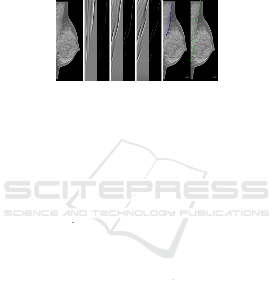
Figure 1: (a) Source image. (b, c, d) Phase response (left) and Laplacian (right) for orientations 180, 170 and 160 respectively.

(e) Detected pectoral muscle boundary (left) marked in blue and ﬁtted line marked in green (right).

1. The three Gabor ﬁlters were each tuned to an ori-

entation (α) of 180, 170 and 160, respectively, to

cover all orientations in which the muscle can ap-

pear.

2. The spatial aspect ratio was set to the value 0.2617

obtained by using the formula

3∗π

2∗M

stated in (Rah-

man and Jha, 2022) with M = 18, where M de-

notes the total number of ﬁlters in the interval

[0, π].

3. The spatial frequency bandwidth was set to 1.2

octaves allowing a moderate range of frequencies

around the central frequency in which the ﬁlter

can respond well.

4. The wavelength (λ) was set in a similar manner

as in (Rahman and Jha, 2022) and was computed

using the formula b

∗

√

c where w denotes the

width of the ROI image to capture high- and mid-

frequency features.

2.1.3 Phase Response of MFG for Pectoral

Muscle Detection

After applying the three Gabor ﬁlters to the ROI im-

age, the phase response of each Gabor response im-

age was computed. To detect and extract the textu-

ral edge information the Laplacian of each phase re-

sponse was computed and combined (addition) (Rah-

man and Jha, 2022). The combined Laplacian image

(Fig. 1b,c,d) was converted into a binary image by ap-

plying simple thresholding with a threshold value of

8. In some cases, a strong intensity edge might be re-

ﬂected in two or three phase responses, and because

of this two or three different intensity edges very close

to each other might appear in the combined Laplacian

(Rahman and Jha, 2022). Morphological closing (ﬁll-

ing small holes) was applied to the resulting image

in order to merge nearby edge lines. The PMB was

obtained by selecting the largest connecting compo-

nent with 8-connectivity. Once the pectoral muscle

had successfully been detected, a line was ﬁtted to the

points on the detected boundary using the linear least

squares method. This is necessary because the actual

PMB is curved, but for computing the PNL length a

straight line is needed (Fig. 1e).

3 NIPPLE DETECTION

3.1 ROI Extraction

For detecting the nipple only a small region is of in-

terest and therefore a small ROI containing the nipple

was extracted. This was done similarly as in (Jiang

et al., 2019). First, the topmost corner marking the

starting point of the breast boundary (x

, y

) com-

puted in ﬁgure 2.1 and the bottom-left corner (x

, y

)

were used as ending points for forming a line. The

angle θ required for rotating this line so that it aligns

with the left image border was calculated

line angle =



tan

−1

(

−y

−x

)



∗

180

(1)

θ = | line angle −90 |. (2)

Then the breast mask computed in ﬁgure 2.1 was

rotated (only necessary for the MLO view) by θ and

passed to the border following algorithm (Suzuki and

Keiichi, 1985) to get the breast contour, the rightmost

point on the contour was identiﬁed and shifted by 35

pixels to the left along the x-axis. A new image with

the same shape as the breast mask ﬁlled with 0-pixels

was then created. Pixel values of pixels lying inside

the rectangular region bounded by the corner points

, 0), (w, 0), (w, h) and (s

, 0) were set to 255 where

, s

) are the coordinates of the shifted point, w is the

width and h is the height of the image. Afterwards,

Automatic Computation of the Posterior Nipple Line from Mammographies

631

(a)

(b)

(c)

(d) (e)

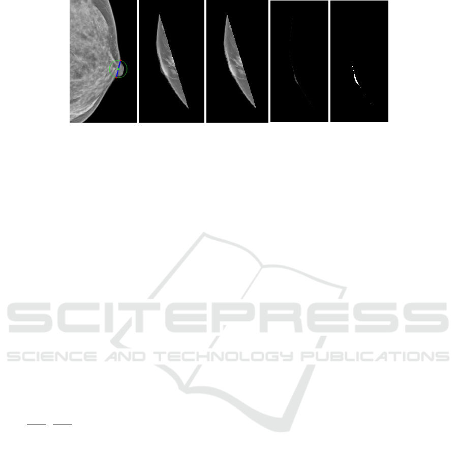
Figure 2: (a) Starting points are marked with red circles and the location of the nipple base is marked with a green circle. (b)

Breast with nipple. (c) Breast without nipple. (d) Output of intersection between (b) and (c). Thresholded image of (d).

bitwise conjunction between the rotated breast mask

and the new image was performed. The new mask

was then rotated back to its original position (only for

the MLO view). To get the ROI containing only the

nipple region bitwise conjunction between the mask

and the source image was performed.

3.2 Detection of the Nipple

First, large nipples that are in proﬁle are located.

Here, the ROI image was converted into a binary

image, and the contour of the nipple region was

computed following the border (Suzuki and Keiichi,

1985). Then the convex hull of the nipple region was

computed which is the minimum boundary that en-

closes this region. Afterwards, the convexity defects

(deviations of the contour from the convex hull), are

calculated. Large deviations with a depth greater than

2.5 usually indicate the starting points of the nipple.

The two points with the largest deviation (x

, y

) and

, y

) were used to ﬁnd the location of the nipple

base (

) (Fig. 2a).

If no deviation with a depth greater than 2.5 was

found, either a small nipple in proﬁle or a subtle nip-

ple was present, a problem that was overcome as ex-

plained next. Usually, small nipples that are in pro-

ﬁle have a distinct nipple base boundary edge and

this characteristic was used to detect them. This was

done by segmenting the nipple from the rest of the

breast using watershed segmentation (Meyer, 1992).

A marker was created by determining which region

belongs to the breast region without the nipple (sure

foreground) and which is the background (sure back-

ground). To obtain the sure background, dilation

(adds pixels to the object boundaries) with a 2 ×2

kernel consisting of ones was applied to the binary

image and for the sure foreground, we applied ero-

sion (removes pixels from boundaries) with a 12 ×12

kernel. By subtracting the sure foreground from the

sure background, a region (unknown) was derived for

which there is no information on whether it belongs

to the foreground or background. This unknown re-

gion encloses the nipple base boundary edge. Next,

the regions in the marker are labelled. The unknown

region was labelled with 0, the background with 1 and

the foreground with 2. The marker was then passed to

the watershed segmentation algorithm to get the con-

tour of the breast region without the nipple. Next, the

intersection between the breast region and the breast

region without the nipple was computed followed by

thresholding. The largest connecting component with

an area greater than 25 was selected as the nipple (Fig.

2).

If no connecting component with an area greater

than 25 was found, a subtle nipple (nipple not in pro-

ﬁle) was present. For detecting subtle nipples the

source image was ﬁrst restricted to the region along

the breast boundary. Next, Non-Local Means Denois-

ing was applied to the ROI image to reduce noise, fol-

lowed by opening (removing small objects from the

foreground) with circular structuring element of size

10 ×10. Afterwards, Hough Circle Transform was

applied to ﬁnd circles with a circle radius between 10

and 25, and only those with a mean intensity greater

than 65 were selected. The ﬁnal subtle nipple is the

circle furthest to the right.

3.3 Posterior Nipple Line Computation

Once the pectoral muscle and nipple have success-

fully been detected, the posterior nipple line and its

length can be computed. Here, the pectoral muscle is

represented as a tuple (m

pec

, c

pec

) where m

pec

is the

slope and c

pec

is the y-intercept in the slope-intercept

form y = m ∗x + c of the pectoral muscle line. If the

muscle line cannot be represented in slope-intercept

form, that is, it is a vertical line, the pectoral muscle

is represented by the variable x

pec

instead, which is

set to the value of the x-coordinate of any point on

that line. The nipple is represented by its coordinates

VISAPP 2024 - 19th International Conference on Computer Vision Theory and Applications

632

(a)

(b)

(c)

(d)

(e)

(f)

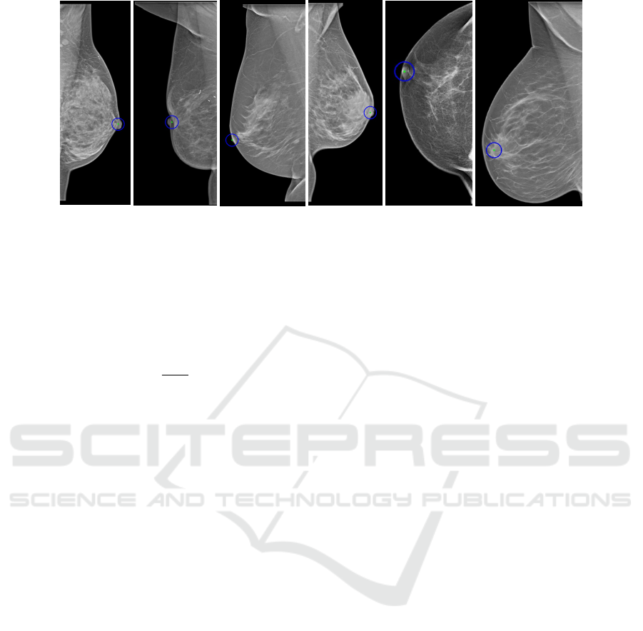
Figure 3: Examples of correctly (a) and falsely (b) located nipples that are in proﬁle and large. Examples of correctly (c) and

falsely (d) located nipples that are in proﬁle and small. Examples of correctly (e) and falsely (f) located nipples that are not in

proﬁle.

nip

, y

nip

In the case where the pectoral muscle is not a ver-

tical line, the slope m

pnl

and the y-intercept c

pnl

of the

linear equation of the PNL were calculated as follows:

pnl

−1

pec

(3)

pnl

= (y

nip

−(m

pnl

∗x

nip

)) (4)

Next, the intersection point (x

inter

, y

inter

) of the

pectoral muscle line and the PNL line was calculated

as follows:



inter





−m

pnl

−m

pec



−1



pnl

pec



(5)

In the case where the pectoral muscle is a vertical

line, the PNL is a horizontal line with linear equation

y = y

nip

and the intersection point is (x

pec

, y

nip

To calculate the length of the PNL, the Euclidean

distance between the intersection point and the nipple

was calculated.

4 EXPERIMENTAL EVALUATION

A dataset of DICOM images provided by the Med-

ical University of Innsbruck was used in our exper-

imental evaluation, which contains mammograms of

both MLO and CC views. For each patient there is an

MLO and a CC view of each breast (left and right),

for some patients, there are only images of one side

of the breast.

4.1 Qualitative Results on Nipple

Detection

Nipples that were large and had well-deﬁned edges at

the two starting points of the nipple were accurately

identiﬁed in most of the cases as shown in ﬁgure 3a.

In cases with no sharp edges, the center could be

slightly off since the points with the largest deviation

can not be accurately deﬁned. Our approach failed

to detect the nipple in rare cases as the one shown in

ﬁgure 3b, which was due to the breast having an in-

dentation at the location of the nipple.

Our approach was also successful at detecting

small nipples that are in proﬁle. This is because the

edge of the nipple base is usually well-deﬁned making

proper segmentation possible (Fig. 3c). If a small nip-

ple in proﬁle was present but the nipple base edge was

not well-deﬁned, our method failed to correctly locate

the nipple (Fig. 3d), but this case rarely occurred.

The detection of nipples that are not in proﬁle

(subtle nipples) is a challenging task even for experts

since in most cases the nipple is not clearly visible or

not visible at all. Therefore the performance of the

proposed method for detecting nipples for this case

was not good. We obtained good results in cases

where the nipple had a round shape and well-deﬁned

edges (Fig. 3e). For cases where the shape of the nip-

ple was not round or its edges were not well-deﬁned,

the Hough Circle Transform failed to accurately iden-

tify the nipple. The center could be slightly off. There

were also some cases where the nipple was not visible

at all (Fig. 3f).

4.2 Qualitative Results on Pectoral

Muscle Detection

The proposed method for pectoral muscle detection

was very accurate for PMBs that have well-deﬁned

edges as in ﬁgure 4a. If dense breast tissue is present

around the border but the edge is still deﬁned, the bor-

der can be still accurately identiﬁed (Fig. 4b). The

Automatic Computation of the Posterior Nipple Line from Mammographies

633

(a)

(b)

(c)

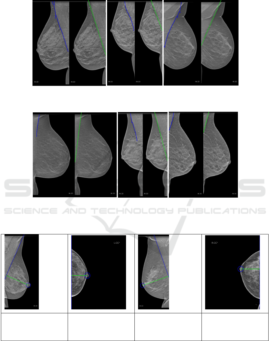
Figure 4: Examples of correctly located PMB. The detected edge is marked in blue and the ﬁtted line to the detected edge is

marked in green.

(a)

(b)

(c)

Figure 5: Examples of falsely located PMB. The detected edge is marked in blue and the ﬁtted line to the detected edge is

marked in green.

Table 1: Examples for computed PNL that were close to the expert values. PNL is marked in green. Values are in mm.

True PNL: 98.90 mm

Computed PNL: 99.72

Difference: 0.82 mm

True PNL: 50.80 mm

Computed PNL: 54.11

Difference: 3.31 mm

True PNL: 114.70 mm

Computed PNL: 114.30

Difference: 0.40 mm

True PNL: 61.40 mm

Computed PNL: 65.15

Difference: 3.75 mm

breast tissue here does not affect our method since it

will be removed during the inpainting step. In ﬁgure

4c the PMB was accurately located even with a occur-

ring fold close to the border. Since the fold has high-

intensity pixels it was removed during the inpainting

step and therefore was not falsely detected as an edge.

There were a few cases where our method failed

to correctly locate the PMB. An example is shown

VISAPP 2024 - 19th International Conference on Computer Vision Theory and Applications

634

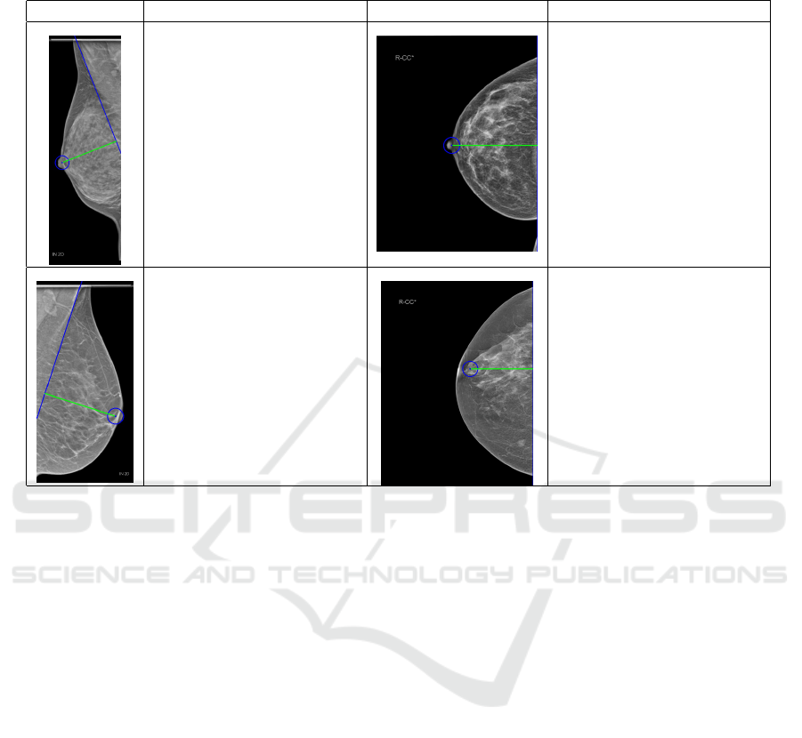
Table 2: Examples for computed PNL that were off when compared to the expert’s. PNL is marked in green. Values are in

mm.

Examples Analysis Examples Analysis

True PNL: 92.00 mm

Computed PNL: 78.41 mm

Difference: 13.59 mm

Here the computed PNL

length is shorter than the

true length. The pectoral

muscle is strongly curved

and therefore the located

boundary is off.

True PNL: 85.90 mm

Computed PNL: 98.61 mm

Difference: 12.71 mm

Here the computed PNL

length is longer than the

true length. The PNL was

measured from the nipple to

the right image border but

should have been measured

from the nipple to the pec-

toral muscle (not visible).

True PNL: 88.80 mm

Computed PNL: 86.56 mm

Difference: 2.24 mm

Here there is a small dif-

ference because the nipple

(in proﬁle and large) was

not located accurately and is

slightly off.

True PNL: 84.80 mm

Computed PNL: 76.54 mm

Difference: 8.26 mm

Here the nipple (not in pro-

ﬁle) was falsely detected,

which led to a large differ-

ence between the actual and

computed PNL length.

in ﬁgure 5a, here the upper part of the PMB could

be accurately identiﬁed since a strong intensity edge

is present, whereas the lower part is strongly blurred

and could not be captured by the Gabor ﬁlters. In this

case, using only the upper part to determine the real

PMB did not sufﬁce. The second example is similar

to the previous one except that the problem lies in the

fact that there was dense breast tissue. Therefore the

detected border was slightly off (Fig. 5b). Another

example of a failure can be seen in ﬁgure 5c, where

multiple edges that are close to each other are present

making it difﬁcult to identify the real PMB. Even if

the PMB can be accurately detected, ﬁtting the line to

the detected edge can still result in a falsely marked

PMB. This is only the case if the actual pectoral mus-

cle is strongly curved.

4.3 PNL Quantitative Results

For evaluating the performance of the proposed

method 100 images from the dataset were used. Im-

ages with breast implants, not visible nipples, or miss-

ing real PNL length (manually measured by an expert

from the Medical University of Innsbruck) were not

considered. The computed PNL length was compared

with the real PNL length. When using those 100 im-

ages, we obtained an absolute mean error of just 6.39

mm (stdev.= 4.62 mm). Since the location of both

the PMB and the nipple are needed for calculating

the PNL length, both of them need to be accurately

located, It would be enough for just one component

to be incorrectly detected to have a negative impact

on the overall performance. In table 1 four examples

(two for each view) with their results can be seen. The

nipples were accurately located in all of them, and the

boundaries of the pectoral muscle were also correctly

identiﬁed in the MLO views. Table 2 shows four ex-

amples of a few cases were results were worse than

expected along with an explanation on the causes.

5 CONCLUSIONS

This thesis presents a method to automatically com-

pute the length of the PNL in mammograms, which

can be divided into three parts: Pectoral Muscle De-

tection, Nipple Detection, and PNL Computation. For

the detection of the PMB, a set of three phase re-

sponses was computed by using three high-frequency

Gabor ﬁlters tuned at three different orientations. The

Laplacian was then computed for each phase response

and combined to detect the muscle boundary. For

the nipple detection method, the convex hull of the

nipple region was used to calculate the convexity de-

Automatic Computation of the Posterior Nipple Line from Mammographies

635

fects. Based on this, a distinction could be made be-

tween large and small nipples. Large nipples can be

located by using the two points with the largest devia-

tion (depth greater than 2.5 each) and small nipples

were located with the help of watershed segmenta-

tion. If no nipple could be found, it means that the

nipple does not lie on the breast boundary and for this

case, Hough Circle Transform was used. Once both

the PMB and nipple were detected, the PNL length

was calculated.

By applying the proposed method on 100 images

from the dataset provided by the Medical Univer-

sity of Innsbruck an absolute mean error of 6.39 mm

could be achieved. In cases where the nipple does not

lie along the breast boundary, the method performs

poorly, but otherwise, the accuracy is high, except for

some rare cases. The overall performance of the de-

tection of the PMB is very accurate, although there is

still room for improvement for some cases.

ETHICS APPROVAL

This study was approved by the ethics commission of

the Medical University of Innsbruck (reference num-

ber 1321/2021).

REFERENCES

Bertalmio, M., Sapiro, G., Caselles, V., and Ballester, C.

(2000). Image inpainting. In Proceedings of the 27th

Annual Conference on Computer Graphics and Interac-

tive Techniques, SIGGRAPH ’00, page 417424, USA.

Brahim, M., Westerkamp, K., Hempel, L., Lehmann, R.,

Hempel, D., and Philipp, P. (2022). Automated assess-

ment of breast positioning quality in screening mammog-

raphy. Cancers, 14(19).

Buades, A., Coll, B., and Morel, J. (2011). Non-Local

Means Denoising. IPOL, 1:208–212.

Deng, J., Dong, W., Socher, R., Li, L., Kai, L., and Li,

F. (2009). Imagenet: A large-scale hierarchical image

database. In CVPR 2009, pages 248–255.

Gupta, V., Taylor, C., Bonnet, S., Prevedello, L., Hawley,

J., White, R., Flores, M., and Erdal, B. (2020). Deep

learning-based automatic detection of poorly positioned

mammograms to minimize patient return visits for repeat

imaging: A real-world application.

Harris, C. and Stephens, M. (1988). A combined corner

and edge detector. In Proceedings of the Alvey Vision

Conference, pages 23.1–23.6. doi:10.5244/C.2.23.

Hejduk, P., Sexauer, R., Ruppert, C., Borkowski, K., Un-

kelbach, J., and Schmidt, N. (2023). Automatic and stan-

dardized quality assurance of digital mammography and

tomosynthesis with deep convolutional neural networks.

Insights into Imaging, 14(1):90.

Jiang, J., Zhang, Y., Lu, Y., Guo, Y., and Chen, H. (2019).

A radiomic-feature based nipple detection algorithm on

digital mammography. Medical Physics, 46.

Klabunde, C., Bouchard, F., Taplin, S., Scharpantgen, A.,

and Ballard-Barbash, R. (2001). Quality assurance for

screening mammography: an international comparison.

JECH, 55(3):204–212.

Meyer, F. (1992). Color image segmentation. In 1992 In-

ternational Conference on Image Processing and its Ap-

plications, pages 303–306.

Pizer, S., Amburn, E., Austin, J., Cromartie, R., Geselowitz,

A., Greer, T., ter Haar Romeny, B., Zimmerman, J., and

Zuiderveld, K. (1987). Adaptive histogram equalization

and its variations. CVGIP, 39(3):355–368.

Rahman, M. and Jha, R. (2022). Multidirectional gabor

ﬁlter-based approach for pectoral muscle boundary de-

tection. IEEE TRPMS, 6(4):433–445.

Sung, H., Ferlay, J., Siegel, R., Laversanne, M., Soerjo-

mataram, I., Jemal, A., and Bray, F. (2021). Global can-

cer statistics 2020: Globocan estimates of incidence and

mortality worldwide for 36 cancers in 185 countries. CA,

71(3):209–249.

Suzuki, S. and Keiichi, A. (1985). Topological structural

analysis of digitized binary images by border following.

CVGIP, 30(1):32–46.

Sweeney, R., Lewis, S., Hogg, P., and McEntee, M. (2017).

A review of mammographic positioning image quality

criteria for the craniocaudal projection. The British jour-

nal of radiology, 91 1082:20170611.

Szegedy, C., Vanhoucke, V., Ioffe, S., Shlens, J., and Wo-

jna, Z. (2015). Rethinking the inception architecture for

computer vision.

Waade, G., Skyrud, D., Holen, A., Larsen, M., Hanestad,

B., Hopland, N., Kalcheva, V., and Hofvind, S. (2021).

Assessment of breast positioning criteria in mammo-

graphic screening: Agreement between artiﬁcial intelli-

gence software and radiographers. Journal of Medical

Screening, 28:096914132199871.

VISAPP 2024 - 19th International Conference on Computer Vision Theory and Applications

636