Fooling Neural Networks for Motion Forecasting via Adversarial Attacks

Edgar Medina

and Leyong Loh

QualityMinds GmbH, Germany

Keywords:

Adversarial Attacks, Human Motion Prediction, 3D Deep Learning, Motion Analyses.

Abstract:

Human motion prediction is still an open problem, which is extremely important for autonomous driving and

safety applications. Although there are great advances in this area, the widely studied topic of adversarial

attacks has not been applied to multi-regression models such as GCNs and MLP-based architectures in human

motion prediction. This work intends to reduce this gap using extensive quantitative and qualitative experi-

ments in state-of-the-art architectures similar to the initial stages of adversarial attacks in image classiﬁcation.

The results suggest that models are susceptible to attacks even on low levels of perturbation. We also show

experiments with 3D transformations that affect the model performance, in particular, we show that most

models are sensitive to simple rotations and translations which do not alter joint distances. We conclude that

similar to earlier CNN models, motion forecasting tasks are susceptible to small perturbations and simple 3D

transformations.

1 INTRODUCTION

Neural networks have demonstrated remarkable capa-

bilities in achieving excellent performance in various

3D tasks, ranging from computer vision to robotics.

Their capacity to process and analyze volumetric data,

point clouds, or 3D meshes has been a driving force

behind their success. Additionally, recent advance-

ments in deep learning techniques, such as Con-

volutional Neural Networks (CNNs), Graph Convo-

lutional Networks (GCNs), and Transformers, have

substantially enhanced their ability to understand and

manipulate 3D data. One notable aspect is their abil-

ity to generalize across different scales, orientations,

and viewpoints has contributed to their robustness in

handling diverse 3D tasks. This robustness is par-

ticularly valuable in scenarios where data may ex-

hibit variations or perturbations, making neural net-

works a valuable tool for applications such as 3D ob-

ject recognition, pose estimation, point cloud analy-

sis, and others. In this work, we combine two dif-

ferent streams of artiﬁcial intelligence. On one side,

deep neural networks have been applied to human

motion prediction in different applications such as

autonomous driving and bioinformatics (Lyu et al.,

2022), (Wu et al., 2022). As mentioned in several pa-

pers, the surprising results of neural network architec-

https://orcid.org/0009-0001-4814-800X

https://orcid.org/0009-0007-7337-3683

tures applied to motion prediction on 3D data struc-

ture surpassed classical approaches (Lyu et al., 2022).

Most of these methodologies are RNN-based family,

GAN-based, mixed multi-linear nets, and GCNs. We

focus mainly on the last two approaches limited to

3D pose forecasting on the Human 3.6M (Ionescu

et al., 2014) dataset, but could be easily extended

to AMASS (Mahmood et al., 2019) and 3DPW (von

Marcard et al., 2018). On the other hand, research

in adversarial attacks has shown that neural networks

are not robust enough for production due to how eas-

ily they are fooled with small perturbations and trans-

formations (Goodfellow et al., 2014), (Xiang et al.,

2019), (Dong et al., 2017). Although adversarial at-

tacks have demonstrated success in fooling GCNs in

recent years (Chen et al., 2021; Liu et al., 2019; Car-

lini and Wagner, 2016; Entezari et al., 2020a; Tanaka

et al., 2021; Diao et al., 2021), these works focus on

classiﬁcation tasks, which are the predominant appli-

cations in machine learning. However, given the na-

ture of our problem, many of these attack methods

are not directly applicable to multi-output regression

tasks. The investigation of adversarial attacks in hu-

man motion prediction is important. One example is

in safety-critical autonomous driving systems, adver-

sarial attacks can cause sensor failure in the pedestrian

motion prediction module of the autonomous vehicle,

consequently resulting in severe accidents. This pa-

per, to the best of our knowledge, presents the ﬁrst

232

Medina, E. and Loh, L.

Fooling Neural Networks for Motion Forecasting via Adversarial Attacks.

DOI: 10.5220/0012562800003660

Paper published under CC license (CC BY-NC-ND 4.0)

In Proceedings of the 19th International Joint Conference on Computer Vision, Imaging and Computer Graphics Theory and Applications (VISIGRAPP 2024) - Volume 4: VISAPP, pages

232-242

ISBN: 978-989-758-679-8; ISSN: 2184-4321

effort of applying adversarial attacks in human mo-

tion prediction and intends to bridge this existing gap

in the literature by conducting extensive experimenta-

tion on different state-of-the-art (SOTA) models.

It is important to highlight a limitation we en-

countered during the progression of our work is the

absence of pre-trained models for several databases.

Since the process of retraining these models using our

own training codes may introduce a noteworthy de-

gree of variability in our experiments, our work in-

volves exclusively working with available pre-trained

models and when corresponding source codes are ac-

cessible to train by ourselves. More concretely, the

experiments involve applying gradient-based attacks

and 3D spatial transformations to neural networks for

multi-output regression tasks in human motion pre-

diction. These experiments exclusively use white-box

attacks because many methodologies adapted directly

to multi-output regression do not yield effective re-

sults. In the preliminary stages of testing, white-box

attacks serve as the initial choice due to their straight-

forward implementation. Conversely, black-box at-

tacks introduce added intricacies when setting up ex-

periments. Also, white-box attacks exhibit elevated

success rates and facilitate the development of more

reﬁned and optimized attack tactics. White-box at-

tacks demonstrate heightened success rates and en-

able the formulation of more precise and reﬁned at-

tack strategies, primarily due to their access to crit-

ical elements such as gradients, loss functions, and

model architecture details. This stands in contrast

to black-box attacks, which initially are resource-

intensive strategies in order to obtain during the itera-

tive process an understanding of the model. This po-

tentially increases the complexity of designing effec-

tive optimization strategies and reduces the precision

if this is not set appropriately. Finally, within the lit-

erature, there is an absence of references to black-box

attacks employed speciﬁcally for multi-output regres-

sion tasks within graph models. We summarize our

contributions as follows:

• We perform extensive experiments on state-of-

the-art models and evaluate the performance im-

pact on the well-studied H3.6M dataset.

• We provide a methodology review for adversarial

attacks applied to human motion prediction.

2 RELATED WORKS

2.1 Adversarial Attacks

Two primary methodologies for adversarial attacks,

namely White-box and Black-box methods, have

been extensively studied in the literature. For the sake

of simplicity and as explained in the introduction sec-

tion, our experiments exclusively were set over white-

box attacks and we excluded black-box methods in

this analysis. In our literature review, we speciﬁcally

focus on graph data, which exhibits parallels with the

pose sequence data we employ. While we acknowl-

edge the considerable impact of white-box attacks

on performance, we also delve into the examination

of 3D spatial transformations as adversarial attacks.

These transformations will be subject to a detailed

comparative analysis in subsequent sections.

White-Box: One of the initial and enduring tech-

niques in image perturbation is the Fast Gradient

Signed Method (FGSM) (Goodfellow et al., 2014),

which relies on computing the gradient through a sin-

gle forward pass of the network. This method sub-

sequently determines the gradient direction through a

sign operation and scales it by an epsilon value be-

fore incorporating it into the current input. Further-

more, an iterative variant (I-FGSM) was introduced

to mitigate pronounced effects when a large epsilon is

used (Goodfellow et al., 2014). More recently, an it-

eration with a momentum factor (MI-FGSM) was in-

troduced into the iterative algorithm, enhancing con-

trol over the gradient and reducing the perceptual vi-

sual impact of the attack (Dong et al., 2017). Iter-

ative approaches have demonstrated their superiority

over one-step methods in extensive experimentation

as robust white-box algorithms, albeit at the expense

of diminished transferability and increased computa-

tional demands (Dong et al., 2019). Later, Carlini

and Wagner’s method (C&W) (Carlini and Wagner,

2016) stands out as an unconstrained optimization-

based technique known for its effectiveness, even

when dealing with defense mechanisms. By har-

nessing ﬁrst-order gradients, this algorithm seeks to

minimize a balanced loss function that simultane-

ously minimizes the norm of the perturbation while

maximizing the distance from the original input to

evade detection. Another relevant method is Deep-

Fool (Moosavi-Dezfooli et al., 2015), which focuses

on identifying the smallest perturbation capable of

causing misclassiﬁcation by a neural network. Deep-

Fool achieves this by linearizing a neural network and

employing an iterative strategy to navigate the hyper-

plane in a simpliﬁed binary classiﬁcation problem.

The minimal perturbation required to alter the clas-

Fooling Neural Networks for Motion Forecasting via Adversarial Attacks

233

siﬁer’s decision corresponds to the orthogonal projec-

tion of the input onto the hyperplane. DeepFool esti-

mates the closest decision boundary for each class and

iteratively adjusts the input in the direction of these

boundaries (Abdollahpourrostam et al., 2023). Im-

portantly, DeepFool is applicable to both binary and

multi-class classiﬁcation tasks.

While there is a wealth of research related to

adversarial attacks in regression tasks (Gupta et al.,

2021), (Nguyen and Raff, 2018), this area remains

relatively unexplored, especially concerning multi-

regression tasks or specialized domains such as 3D

pose forecasting. Despite the signiﬁcant progress

in adversarial attacks, the majority of methods have

mainly been applied to classiﬁcation tasks. Therefore,

we introduce a mathematical framework for regres-

sion tasks to address this gap in research.

Adversarial Attacks on Graph Data: The out-

put of pose estimation can be regarded as graph

data, contingent on its structure and representation.

Poses contain 2D or 3D positions, also called key-

points or joints, of the human body connected by a

skeleton. Numerous prior studies within this domain

have extensively explored gradients and their appli-

cation in classiﬁcation tasks (Sun et al., 2018; Zhang

et al., 2020; Fang et al., 2018; Zhu et al., 2019; Liu

et al., 2019; Carlini and Wagner, 2016; Entezari et al.,

2020a; Tanaka et al., 2021; Diao et al., 2021; Z

ugner

et al., 2020). In our work, we take these studies as in-

spiration to implement our approach in multi-output

regression. In the next section, we provide more de-

tails about working with multiple real-valued outputs

given that the target is not a binary output the methods

must be adapted in this work. Furthermore, defense

strategies previously studied in (Chen et al., 2021)

and (Entezari et al., 2020b) showed that the attack ef-

fects can be reduced, however, these approaches are

beyond the scope of this work.

3D Point Cloud Operations: Taking inspiration

from prior research on adversarial attacks in point

clouds (Dong et al., 2017), we explore geometric

transformations applied to 3D data points. Our ob-

jective is to manipulate these data points while pre-

serving their distance distributions (Sun et al., 2021;

Huang et al., 2022; Hamdi et al., 2019; Dong et al.,

2017). Notably, many of these previous works em-

ploy metrics such as Hausdorff distance and distribu-

tion metrics rather than MPJPE to quantify discrepan-

cies between the adversarial input and the original in-

put. Our experiments revolve around spatio-temporal

afﬁne transformations, including rotation, translation,

and scaling, as a means to modify the pose sequences.

2.2 3D Pose Forecasting

In this section, we investigate various architectural

paradigms, including GCNs, RNN-based models, and

MLP-based models (Lyu et al., 2022), that have been

employed for human motion prediction. During the

preprocessing stage, some models adopt Discrete Co-

sine Transforms (DCT) to transform the 3D input data

into the frequency domain. This approach draws in-

spiration from prior work in graph processing, as dis-

cussed in (Sun et al., 2018). There are branches re-

lated to how the 3D input data is used: pre-processed

and original.

Using a pre-processed input approach in the con-

text of 3D pose prediction, DCT has been employed

by (Guo et al., 2022), (Ma et al., 2022), (Mao et al.,

2020), and (Mao et al., 2021) to encode the input se-

quence. This encoding method is designed to capture

the periodic body movements inherent in human mo-

tion. These studies showed substantial improvements

in model predictions, surpassing the performance of

previous RNN-based approaches. However, this op-

eration is not only computationally expensive but also

needs the use of Inverse DCT (IDCT) to revert the

data back to the Euclidean space. Alternatively, other

preprocessing approaches propose the replacement of

input data or the aggregation of instantaneous dis-

placements and displacement norm vectors (Bouaz-

izi et al., 2022; Guo et al., 2022). These methodolo-

gies have shown a notable reduction in error metrics.

However, the pioneering network that, as far as our

knowledge, directly incorporates the original 3D data

into the model is called Space-Time-Separable Graph

Convolutional Network (STS-GCN) (Soﬁanos et al.,

2021).

The current SOTA models in the ﬁeld encompass

MotionMixer (Bouazizi et al., 2022), siMLPe (Guo

et al., 2022), STS-GCN (Soﬁanos et al., 2021), PG-

BIG (Ma et al., 2022), HRI (Mao et al., 2020), and

MMA (Mao et al., 2021). MotionMixer and siMLPe

are both MLP-based models that borrow the idea of

Mixer architecture (Tolstikhin et al., 2021) and ap-

ply it to the domain of human pose forecasting. STS-

GCN and PGBIG are founded on GCNs. STS-GCN

utilizes two successive GCNs to sequentially encode

temporal and spatial pose data, while PGBIG intro-

duces a multi-stage prediction framework with an it-

erative reﬁning of the initial future pose estimate for

improved prediction accuracy. HRI and MMA are

GCN-based models augmented with attention mod-

ules. HRI introduces a motion attention mechanism

based on DCT coefﬁcients, which operate on sub-

sequences of the input data. MMA takes a distinctive

approach by employing an ensemble of HRI models

VISAPP 2024 - 19th International Conference on Computer Vision Theory and Applications

234

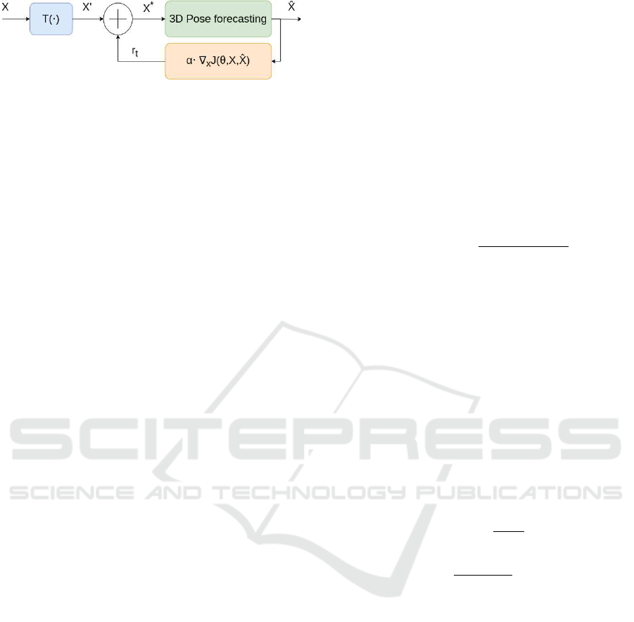
Figure 1: General diagram block for our experiments.

at three different levels: full-body, body parts, and in-

dividual joints, to achieve enhanced prediction accu-

racy. In contrast to other SOTA models, MotionMixer

adopts pose displacements as its input representation,

whereas PGBIG, siMLPe, HRI, and MMA utilize

DCT encoding for the input pose data. Tab. 1 and Tab.

2 present the action-wise and average MPJPE results

for the SOTA models on the Human3.6M dataset.

3 METHODOLOGY

3.1 Mathematical Notation

Let X be the input pose sequence and

X the out-

put pose sequence. Every pose sequence belongs to

T ×J×D

where T J, and D are the temporal, joint

domains and the 3D Euclidean positions respectively.

Furthermore, we denote X

and X

∗

as the transformed

and the adversarial examples for an input pose. This

formulation process is visually depicted in Fig. 1. It

is important to observe that an identity transforma-

tion means that the transformed variable X

would be

identical to the original variable X.

3.2 Gradient-Based Methods

We ﬁrst detail a commonly used non-targeted attack

called FGSM algorithm. FGSM ﬁnds an adversarial

example X

∗

that maximizes the loss function L(θ,x,y)

composed by L

∞

norm of the difference which is lim-

ited to a small ε. This is expressed in Eq. 1.

∗

= X +ε·sign(∇

L(θ,x, y)), kX

∗

−Xk

∞

≤ ε (1)

The iterative extension of FGSM, known as

IFGSM, applies the fast gradient method for multi-

ple iterations, introducing incremental changes con-

trolled by a scaling factor denoted as α. Conse-

quently, the adversarial example X

∗

is updated itera-

tively for a total of t times as described in Eq. 2, where

represents the adversarial example at the t-th iter-

ation. It is essential to emphasize that, as outlined in

(Dong et al., 2017), X

∗

must satisfy the boundary con-

dition imposed by ε to ensure minimal perturbation,

as denoted by kX

∗

−Xk ≤ ε within the algorithm. The

choice of norm for this constraint typically includes

the L

, L

, and L∞ norms. An alternative represen-

tation for the perturbation factor α can be derived by

setting α = ε/T , where T is the total number of itera-

tions.

∗

= X, X

∗

t+1

= X

∗

+ α · sign(∇

∗

L(θ,x, y)) (2)

A more sophisticated variant of IFGSM has been

proposed to improve the transferability of adversarial

examples by incorporating momentum within the iter-

ative process. The update procedure is shown in Eqs.

3 and 4, where g

gathers the gradient information in

the t-th iteration, subject to a decay factor µ.

t+1

= µ · g

∇

∗

L(θ,x, y)

k∇

∗

L(θ,x, y)k

(3)

∗

t+1

= X

∗

+ α · sign(g

t+1

) (4)

The DeepFool approach merges a linearization

strategy with the vector projection of a given sample.

This projection corresponds to the minimum distance

required to cross the hyperplane in the context of bi-

nary classiﬁcation. Subsequently, this approach has

been extended to multi-class classiﬁcation scenarios.

The noise introduced is described as a vector projec-

tion originating from a point x

, oriented in the di-

rection of the hyperplane’s normal vector W , with the

distance serving as its magnitude. This mathemati-

cal representation is expressed in Eq. 5. However,

with the iterative application of noise, its representa-

tion evolves as shown in Eq. 6.

∗

) = −

f (x

)

kwk

w (5)

← −

f (x

)

k∇ f (x

∇ f (x

) (6)

Our methodology comprises two primary steps.

First, we establish a neural network linearization ap-

proach, similar to previous methodologies explored in

works such as (Moosavi-Dezfooli et al., 2015; Gupta

et al., 2021; Nguyen and Raff, 2018). Second, we

introduce a noise vector to the point x

, strategically

positioned to be in very close proximity to the hy-

perplane Π : W

X. This is illustrated in Fig. 2.

This noise vector must have a horizontal orientation

to ensure that an input changes, transitioning from

X ∈ R

xJx3

X ∈ R

xJx3

, does not induce any alter-

ations in the output y ∈ R

xJx3

. This condition can be

mathematically expressed as a straightforward regres-

sion problem, namely y = f

), where typically T

and T

differ. Also, it becomes evident from the ﬁgure

that the error denoted as E is directly proportional to

the magnitude of the noise vector kr

k. For instance,

Fooling Neural Networks for Motion Forecasting via Adversarial Attacks

235

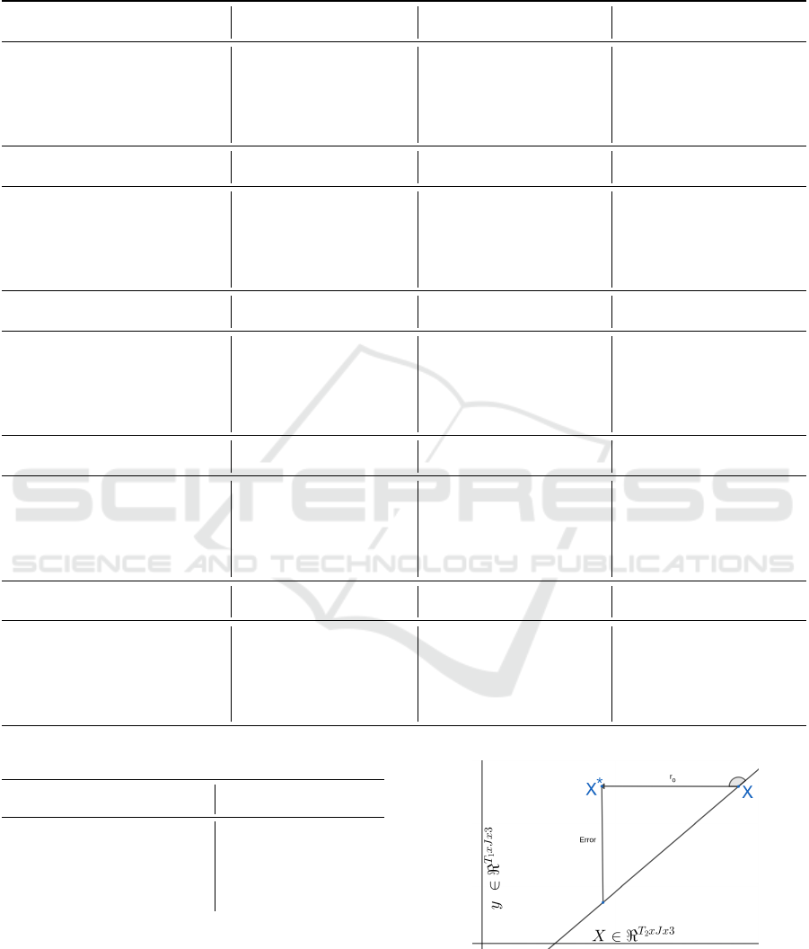
Table 1: Action-wise performance comparison of MPJPE for motion prediction on Human3.6M. We employ our evaluation

pipeline only for the 1000ms models. A notable discrepancy exists between our evaluation results and those reported in the

original papers. This variation is mainly due to the original papers using different strategies and frame evaluations.

Walking Eating Smoking

Time (ms) 80 160 320 400 560 1000 80 160 320 400 560 1000 80 160 320 400 560 1000

STS-GCN (Soﬁanos et al., 2021) 18.0 32.9 46.7 53.4 58.0 70.2 12.1 23.3 36.8 44.3 57.4 82.6 13.0 16.4 37.2 44.6 55.5 76.1

PGBIG (Ma et al., 2022) 14.5 34.5 66.7 79.0 96.7 111.2 7.93 19.2 38.9 48.0 63.8 88.7 8.55 20.0 39.7 48.1 62.0 85.5

MotionMixer (Bouazizi et al., 2022) 14.4 27.0 46.2 52.7 58.7 66.1 8.5 17.3 33.5 41.3 54.4 79.9 9.0 17.9 34.3 41.7 53.2 74.3

siMLPe (Guo et al., 2022) 12.0 20.5 34.8 40.2 48.7 57.3 9.9 16.2 30.4 37.6 53.4 79.1 10.5 17.0 31.5 38.0 51.4 73.9

HRI (Mao et al., 2020) 10.0 19.5 34.2 39.8 47.4 58.1 6.4 14.0 28.7 36.2 50.0 75.6 7.0 14.9 29.9 36.4 47.6 69.5

MMA (Mao et al., 2021) 9.9 19.3 33.8 39.1 46.2 57.2 6.2 13.7 28.1 35.3 48.7 73.8 6.8 14.5 29.0 35.5 46.5 68.8

Discussion Directions Greeting

Time (ms) 80 160 320 400 560 1000 80 160 320 400 560 1000 80 160 320 400 560 1000

STS-GCN (Soﬁanos et al., 2021) 17.1 33.2 58.6 71.3 91.1 118.9 13.9 29.3 52.8 64.0 79.9 109.6 20.8 40.7 72.2 85.9 106.3 136.1

PGBIG (Ma et al., 2022)

12.1 28.7 58.5 71.6 93.6 123.9 9.1 23.0 49.8 61.4 77.7 108.9 16.2 38.0 74.6 88.6 111.1 143.8

MotionMixer (Bouazizi et al., 2022) 12.7 27.1 56.8 70.2 91.7 123.8 9.0 20.9 48.1 60.2 76.9 110.1 16.6 35.5 72.7 87.5 110.8 145.6

siMLPe (Guo et al., 2022) 12.5 24.6 52.2 65.2 87.8 118.8 11.2 20.4 45.7 57.2 76.3 110.1 15.1 30.2 63.5 77.8 101.3 139.3

HRI (Mao et al., 2020) 10.2 23.4 52.1 65.4 86.6 119.8 7.4 18.4 44.5 56.5 73.9 106.5 13.7 30.1 63.8 78.1 101.9 138.8

MMA (Mao et al., 2021) 9.9 22.9 51.0 64.0 85.3 117.8 7.2 18.0 43.3 55.0 72.3 105.8 13.6 30.0 63.2 77.5 101.0 137.9

Phoning Posing Purchases

Time (ms) 80 160 320 400 560 1000 80 160 320 400 560 1000 80 160 320 400 560 1000

STS-GCN (Soﬁanos et al., 2021) 14.5 27.3 45.7 55.4 73.1 108.3 19.0 38.9 71.7 89.2 119.7 178.4 20.9 41.4 71.8 86.0 106.8 141.0

PGBIG (Ma et al., 2022) 10.2 23.5 48.5 59.3 77.6 114.4 12.3 30.6 66.2 82.1 111.0 173.8 14.8 34.2 65.5 78.4 99.3 136.7

MotionMixer (Bouazizi et al., 2022) 10.5 21.2 43.6 54.2 72.6 110.1 12.6 28.3 65.0 82.5 113.4 181.3 15.3 33.5 67.8 81.7 102.6 143.7

siMLPe (Guo et al., 2022) 11.8 19.9 39.8 49.4 68.2 103.7 13.4 25.8 58.8 74.8 105.9 170.0 15.6 29.9 60.0 73.5 96.5 135.4

HRI (Mao et al., 2020) 8.6 18.3 39.0 49.2 67.4 105.0 10.2 24.2 58.5 75.8 107.6 178.2 13.0 29.2 60.4 73.9 95.6 134.2

MMA (Mao et al., 2021) 8.5 18.0 38.3 48.4 66.6 104.1 9.8 23.7 58.0 75.1 105.8 171.5 12.8 28.7 59.5 72.8 94.6 133.6

Sitting Sitting Down Taking Photo

Time (ms) 80 160 320 400 560 1000 80 160 320 400 560 1000 80 160 320 400 560 1000

STS-GCN (Soﬁanos et al., 2021) 16.0 30.1 51.9 63.9 84.7 121.4 23.9 42.9 68.9 81.5 105.2 148.4 16.2 31.3 52.1 63.4 84.2 126.3

PGBIG (Ma et al., 2022) 10.0 22.2 45.5 56.3 76.2 114.4 15.8 33.5 61.8 74.1 98.5 143.3 9.3 21.3 44.6 55.5 75.7 116.1

MotionMixer (Bouazizi et al., 2022) 10.8 22.4 46.5 57.8 78.0 116.4 17.1 34.6 64.3 77.7 103.3 149.6 9.6 20.3 43.5 54.5 75.3 118.3

siMLPe (Guo et al., 2022) 13.2 22.2 45.5 56.8 79.3 118.2 18.3 32.4 59.8 72.3 99.2 144.8 12.5 20.5 41.6 52.1 73.8 114.1

HRI (Mao et al., 2020) 9.3 20.1 44.3 56.0 76.4 115.9 14.9 30.7 59.1 72.0 97.0 143.6 8.3 18.4 40.7 51.5 72.1 115.9

MMA (Mao et al., 2021) 9.1 19.7 43.7 55.5 75.8 114.6 14.7 30.4 58.5 71.4 96.2 142.0 8.2 18.1 40.2 51.1 71.8 114.6

Waiting Walking Dog Walking Together

Time (ms) 80 160 320 400 560 1000 80 160 320 400 560 1000 80 160 320 400 560 1000

STS-GCN (Soﬁanos et al., 2021) 15.9 31.5 52.3 63.4 80.8 113.6 29.2 53.3 84.2 96.1 115.4 151.5 15.5 28.2 42.3 49.9 58.9 72.5

PGBIG (Ma et al., 2022) 10.6 25.2 53.1 65.2 83.8 113.1 22.5 47.2 81.1 93.6 113.8 151.4 11.5 28.0 55.2 66.7 83.0 99.0

MotionMixer (Bouazizi et al., 2022) 10.8 22.8 49.1 61.0 80.3 113.4 24.2 47.2 81.0 93.0 111.6 153.8 11.6 23.1 43.5 51.7 61.2 69.9

siMLPe (Guo et al., 2022) 11.5 20.6 43.7 54.2 74.0 106.1 22.3 40.7 72.6 85.0 108.7 145.0 11.8 19.9 35.7 42.1 53.7 64.6

HRI (Mao et al., 2020) 8.7 19.2 43.4 54.9 74.5 108.2 20.1 40.3 73.3 86.3 108.2 146.8 8.9 18.4 35.1 41.9 52.7 64.9

MMA (Mao et al., 2021) 8.4 18.8 42.5 53.8 72.6 104.8 19.6 39.5 71.8 84.3 105.1 142.1 8.5 17.9 34.4 41.2 51.3 63.3

Table 2: Average MPJPE for H3.6M dataset.

Average

Time (ms) 80 160 320 400 560 1000

STS-GCN (Soﬁanos et al., 2021) 17.7 33.9 56.3 67.5 85.1 117.0

PGBIG (Ma et al., 2022) 12.4 28.6 56.7 68.5 88.2 121.6

MotionMixer (Bouazizi et al., 2022) 12.8 26.6 53.1 64.5 82.9 117.1

siMLPe (Guo et al., 2022) 13.4 24.0 47.7 58.4 78.6 112.0

HRI (Mao et al., 2020) 10.4 22.6 47.1 58.3 77.3 112.1

MMA (Mao et al., 2021) 10.2 22.2 46.4 57.3 76.0 110.1

when considering an angle of 45

◦

within a right tri-

angle, the error magnitude aligns with the magni-

tude of the noise vector. This observation means that

networks with heightened susceptibility, particularly

from a numerical instability perspective, are more

likely to exhibit larger errors.

Figure 2: Visual interpretation of an algorithm for regres-

sion tasks.

3.3 Spatio-Temporal Transformations

In contrast to adding noise into the pose sequences,

we propose an alternative approach involving the ap-

VISAPP 2024 - 19th International Conference on Computer Vision Theory and Applications

236

plication of 3D transformations, speciﬁcally afﬁne

transformations, to evaluate the models. The gen-

eral form of an afﬁne transformation in homogeneous

coordinates is mathematically represented in Eq. 7,

where A represents the afﬁne matrix, and t is the

translation vector. The matrix A implicitly contains

both the rotation matrix and the scaling factor through

a matrix multiplication operation between these two

matrices. The output of the transformation, denoted

as X

, is obtained after operating the transformation

T (·). Hence, the ﬁnal adversarial example is derived

through the addition of noise r

, as illustrated in Fig.

1. This process is formally expressed in Eqs. 8 and

9. It is worth noting that the transformation operation

T (·) may behave as an identity matrix in certain cases.

H =



A t



,where detA 6= 0 (7)

= T (X) (8)

∗

= X

+ r

(9)

4 EXPERIMENTATION

4.1 Datasets

We conducted experiments on the Human 3.6M

(Ionescu et al., 2014) dataset. This dataset consists of

a diverse set of 15 distinct actions performed by 7 dif-

ferent actors. To facilitate consistent processing, we

downsampled the frame rate to 25Hz and employed a

22-joint conﬁguration same as in (Mao et al., 2020)

and (Fu et al., 2022). It means subjects 1, 6, 7, 8, and

9 were set for training, subject 11 for validation, and

subject 5 for testing.

4.2 Results

We have opted to select SOTA models for our exper-

iments. To ensure a fair comparison, we have uni-

formly implemented all these models within our eval-

uation pipeline and have evaluated them using a con-

sistent standard metric. These experiments serve to

analyze the impact of adversarial attacks and spatial

transformations on the performance of these models,

thereby providing valuable insights into the strengths

and limitations of various architectures. We also at-

tempted to conduct experiments with AMASS and

3DPW datasets. However, we encountered a chal-

lenge as there were no training codes or pre-trained

Figure 3: Result of FGSM with increasing epsilon on aver-

age MPJPE.

models available for all the models. Also, conduct-

ing a fair and meaningful comparison across all mod-

els under these conditions was rendered infeasible.

Therefore, only STS-GCN, MotionMixer and siMLPe

are evaluated on AMASS and 3DPW.

Metric. In our evaluations, we employ the Mean

Per Joint Position Error (MPJPE) metric, which is a

widely accepted evaluation measure commonly used

in previous works (Lyu et al., 2022; Dang et al., 2021;

Liu et al., 2021) to compare two pose sequences. The

MPJPE metric is deﬁned in Eq. (10).

MPJPE

J × T

∑

t=1

∑

j=1

k ˆx

j,t

− x

j,t

(10)

Quantitative Results. We conducted adversar-

ial attacks using the IFGSM, MIFGSM, and Deep-

Fool techniques on the SOTA models. Tabs. 3 and

4 present the outcomes of these adversarial attacks

when applied to the models on the Human 3.6M

dataset. The variable ∆s represents the Euclidean

distance between the adversarial examples and their

corresponding real examples, and w/o represents the

original average MPJPE without any attack.

Fig. 3 shows the effect of epsilon on average

MPJPE, similar effect occurred in our experiment for

IFGSM and MIFGSM. We therefore ﬁxed the ε value

for our experiments in Tabs. 3 and 4 at 0.001 and 0.01.

Another reason for that was because of the increase

of ∆s as average MPJPE increases. The goal of the

adversarial attacks is to keep ∆s as small as possible

but to maximize average MPJPE. When ∆s becomes

too large, it becomes infeasible to occur in reality. In

terms of number of iterations it was speciﬁed as 10

for IFGSM, MIFGSM, and DeepFool. The parameter

µ in MIFGSM was set to 0.4. DeepFool has only one

parameter, the number of iterations.

We highlight that previous attempts at adversarial

attacks were mostly applied to images, which typi-

Fooling Neural Networks for Motion Forecasting via Adversarial Attacks

237

Table 3: Comparison of adversarial attacks on average MPJPE for H3.6M. The arrows denote superior results. (ε = 0.001).

Model IFGSM (↑) ∆s (↓) MIFGSM (↑) ∆s (↓) DeepFool (↑) ∆s (↓) w/o

STS-GCN 86.1 (+16%) 1.3 86.1 (+16%) 1.3 89.5 (+20%) 2.6 74.7

PGBIG 96.9 (+28%) 0.3 96.2 (+27%) 0.3 86.7 (+15%) 0.9 75.2

MotionMixer 72.3 (+1%) 0.02 72.3 (+1%) 0.02 101.9 (+43%) 2.6 71.2

siMLPe 131.3 (+94%) 1.1 133.1 (+97%) 1.2 86.9 (+29%) 0.9 67.5

HRI 115.2 (+73%) 1.2 113.8 (+71%) 1.2 82.1 (+24%) 0.7 66.4

MMA 107.1 (+64%) 1.2 105.9 (+62%) 1.2 79.7 (+22%) 0.7 65.3

Table 4: Comparison of adversarial attacks on average MPJPE for H3.6M. The arrows denote superior results. (ε = 0.01).

Model IFGSM (↑) ∆s (↓) MIFGSM (↑) ∆s (↓) DeepFool (↑) ∆s (↓) w/o

STS-GCN 239.5 (+220%) 13.1 236.2 (+216%) 13.5 89.5 (+20%) 2.6 74.7

PGBIG 173.7 (+131%) 2.3 178.2 (+137%) 2.6 86.7 (+15%) 0.9 75.2

MotionMixer 84.1 (+18%) 0.2 83.9 (+17%) 0.2 101.9 (+43%) 2.6 71.2

siMLPe 281.1 (+316%) 10.7 296.6 (+339%) 11.5 86.9 (+29%) 0.9 67.5

HRI 264.1 (+297%) 11.5 274.0 (+312%) 12.1 82.1 (+24%) 0.7 66.4

MMA 250.8 (+284%) 11.7 259.7 (+297%) 12.2 79.7 (+22%) 0.7 65.3

Table 5: Comparison of adversarial attacks on the average MPJPE for AMASS. The arrows denote superior results. (

∗

) model

was trained by us. (ε = 0.01).

Model IFGSM (↑) ∆s (↓) MIFGSM (↑) ∆s (↓) DeepFool (↑) ∆s (↓) w/o

STS-GCN 194.8 (+78%) 12.2 194.8 (+78%) 12.2 119.6 (+9%) 4.3 109.6

MotionMixer 89.1 (+1%) 0.17 89.1 (+1%) 0.17 89.0 (+1%) 2.6 88.5

siMLPe

∗

189.8 (+406%) 12.5 190.2 (+407%) 12.5 66.9 (+78%) 1.3 37.5

Table 6: Comparison of adversarial attacks on average MPJPE for 3DPW. The arrows denote superior results. (

∗

) model was

trained by us. (ε = 0.01).

Model IFGSM (↑) ∆s (↓) MIFGSM (↑) ∆s (↓) DeepFool (↑) ∆s (↓) w/o

STS-GCN 190.4 (+79%) 13.7 190.2 (+79%) 13.7 115.5 (+9%) 4.3 106.1

MotionMixer 69.5 (+1%) 0.19 69.5 (+1%) 0.19 69.0 (+0%) 2.5 69.0

siMLPe

∗

189.5 (+358%) 12.4 190.0 (+360%) 12.3 63.7 (+54%) 1.3 41.3

cally have pixel values normalized to the range be-

tween 0 and 1. However, in our case, we are apply-

ing adversarial attacks to 3D human pose sequences,

which consist of real numbers larger than 1. There-

fore, to determine the actual ε value for each sample,

we scaled the predeﬁned epsilon value using the ex-

pression from Eqs. 1, 2, and 4, while considering the

vertical axis, as indicated by the term |X

max

− X

min

This approach ensures that the added perturbation re-

mains within a reasonable and meaningful range.

As shown in Tabs. 3 and 4, MotionMixer stands

out as the most robust model in comparison to the oth-

ers. This heightened robustness can be attributed to

the utilization of pose displacements as input data,

while other models rely on pose positions or pre-

processed versions of these. Consequently, by incor-

porating changes in pose positions between consec-

utive frames as input, we increase the robustness of

the model. In our ablation study, we explore the im-

pact of the parameter µ in the MIFGSM method on

the MPJPE. Fig. 4 reveals that the optimal µ value

falls within the range of 0.25 to 0.5, which consis-

tently yields the largest average MPJPE error across

all models. We also noted that the input sequences

vary in length among our models, and this varia-

tion can also impact the gradient magnitude, adding

an additional layer of complexity to our analysis.

Also, to demonstrate the performance and generaliza-

tion capabilities of these attacks. We also apply the

same IFGSM, MIFGSM, and DeepFool algorithms to

available SOTA models for the AMASS and 3DPW

datasets, this is presented in Tabs. 5 and 6 respec-

tively. As we can observe, MotionMixer reﬂects the

best robustness against attacks. We indicate with (

∗

)

to point to the models that were trained by us using

the author’s codes.

In addition to conventional adversarial attacks, we

have introduced spatial perturbations to our models

and evaluated their performance based on the MPJPE.

As depicted in Fig. 5, STS-GCN exhibits sensitivity

VISAPP 2024 - 19th International Conference on Computer Vision Theory and Applications

238

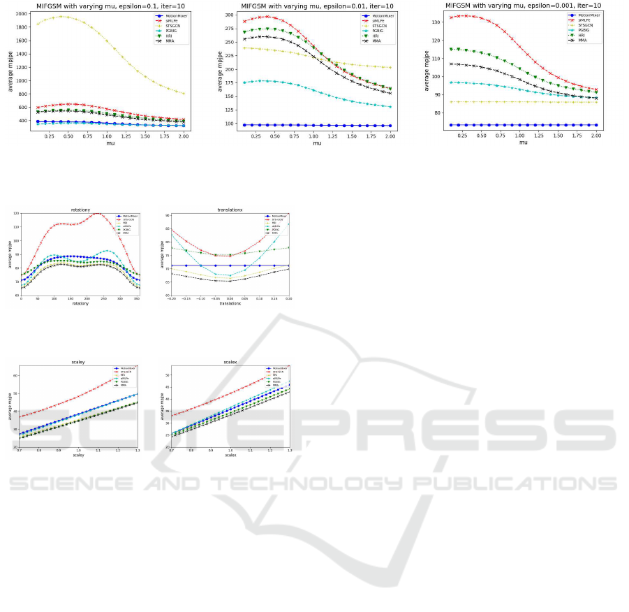
(a) ε equal to 0.1 (b) ε equal to 0.01 (c) ε equal to 0.001

Figure 4: Result of MIFGSM on average MPJPE with µ ranging from 0.0 to 2.0 with granularity 0.1 using 10 iterations.

(a) Rotations between 0-360

degrees in the Y-axis

(b) Scale rate between 0.7

and 1.3 in the Y-axis

-0.2 and 0.2 in the X-axis

(d) Scale rate between 0.7

and 1.3 in the X-axis.

Figure 5: Transformation effects on the test set using the

average MPJPE over the 25 output frames.

to spatial perturbation, primarily due to its higher gra-

dient (rate of change concerning perturbation) com-

pared to other models. On the other hand, Motion-

Mixer, which utilizes pose displacements as input,

displays a robust behavior to rotation and translation

perturbations, as these alterations have minimal im-

pact on the performance following 3D transforma-

tions. For this reason, MotionMixer behaves as the

most robust architecture against translation perturba-

tion, as reﬂected by the nearly ﬂat average MPJPE,

which remains unchanged for different translation

factors applied to the input. Finally, we conducted ex-

periments involving scale transformations to demon-

strate that the MPJPE performance does not exhibit

a linear increase for all models in a uniform manner.

Although we know that the MPJPE metric is inﬂu-

enced by the scale factor, we observe that the model

predictions are also not accurately scaled. All the tests

presented in this context can be considered as out-of-

distribution data.

Qualitative Results. In order to show visually the

effect of the adversarial attacks on the models. In Fig.

6, we visualize the output of the SOTA models for a

“walking” motion in the following order: HRI, MMA,

MotionMixer, PGBIG, STSCGN, and siMLPe. We

show the effect of rotation over the vertical axis and

how this affects the model performance. More de-

tailed, Fig. 6a shows the original prediction while Fig.

6b shows the prediction for a rotated input. The plot

shows the samples with predictions of 80, 160, 320,

400, 560, 720, 880, and 1000 ms. Additionally, we

also present in Fig. 7 the output prediction of STS-

GCN before (ﬁrst row) and after applying the IFGSM

algorithm for different epsilon values. We show the

output prediction at timestamps of 80, 160, 320, 400,

560, 720, 880, and 1000 ms. The average MPJPE for

this “walking” sample is originally 48.35 but after ap-

plying IFGSM, the values average MPJPE are 53.30,

109.08, and 592.89 for epsilon values at 0.001, 0.01,

and 0.1. We know that epsilon at 0.1 is large enough

to fool the network but have a cost on the ∆s in the

input domain. Visually we can observed a prediction

collapse for ε equal to 0.1 in Fig. 7. We also un-

derstand that in regression, numerical stability has a

large cost when these attack algorithms are applied.

But with a deﬁned metric for the difference between

the input and adversarial samples ∆s, we could use

this controlled noise in the training stage.

5 DISCUSSION

Despite conducting an extensive array of experi-

ments employing SOTA models on well-established

datasets, we observed that the prediction error re-

mained nearly consistent across all frames. This phe-

nomenon can be attributed to the threshold imposed

by the FGSM algorithm family. However, Deepfool,

which utilizes the output predictions and processes

them with their gradients, allows for the generation

of a non-ﬂat response when introducing adversarial

Fooling Neural Networks for Motion Forecasting via Adversarial Attacks

239

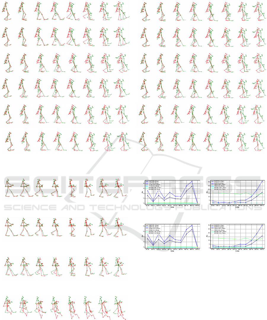
(a) Original input. (b) Rotation 240

◦

in the vertical axis.

Figure 6: Prediction for a walking pedestrian before and after rotating 240

◦

(a) original

(b) ε = 0.001

(d) ε = 0.1

Figure 7: Prediction for a walking pedestrian after applying

an adversarial attack.

noise. To apply Deepfool effectively in our context

with pose sequences, certain adaptations were needed

due to disparities in input and output shapes. In con-

(a) MotionMixer on 3DPW (b) STSGCN on 3DPW

Figure 8: Adversarial attacks applied to STSGCN and Mo-

tionMixer models on the AMASS and 3DPW datasets.

trast to Deepfool, FSGM uses gradients that have the

same shape as the input sequence. Consequently, our

approach takes the average of the output gradients

in the time domain, which was subsequently prop-

agated as a single-frame error. This adaptation re-

sulted in a distinct gradient behavior. This is illus-

trated in Fig. 8 for AMASS and 3DPW datasets,

where the horizontal axis presents the frame index

and the vertical axis presents the difference between

the original and adversarial sequences, denoted as ∆s.

We use the mean Hausdorff distance metric for Mo-

tionMixer and the MPJPE metric for STS-GCN. This

choice was made to see more insightful visualiza-

VISAPP 2024 - 19th International Conference on Computer Vision Theory and Applications

240

tions, particularly considering that MotionMixer em-

ploys displacement-based representations with values

that are typically very low. It can be observed that the

adversarial attacks algorithms learn to exert the most

variation in ∆s to the last frame, in order to fool the

models. Additionally, in the case of MotionMixer, the

last displacement is replaced with the positions of the

last frame for this evaluation, that’s why the ∆s drop

to zero for the last displacement frame.

6 CONCLUSIONS AND FUTURE

DIRECTION

We observed that models are easily fooled by adver-

sarial attacks as same as in the initial stages of CNNs

on image classiﬁcation. Furthermore, we showed

that 3D spatial transformations also behave as no-

gradient-based attack methods and have strong ef-

fects on the model performance. As a future direc-

tion, we plan to use these methods as data augmenta-

tion for more realistic scenarios such as small short-

period rotations or spatio-temporal windowed noise.

We also plan to explore black-box methods since we

observed white-box attacks worked successfully and

also a white-box method using the gradients to guide

the 3D spatial transformations.

ACKNOWLEDGEMENTS

The research leading to these results is funded by the

German Federal Ministry for Economic Affairs and

Climate Action within the project “ATTENTION –

Artiﬁcial Intelligence for realtime injury prediction”.

The authors would like to thank the consortium for

the successful cooperation.

REFERENCES

Abdollahpourrostam, A., Abroshan, M., and Moosavi-

Dezfooli, S.-M. (2023). Revisiting DeepFool: gen-

eralization and improvement.

Bouazizi, A., Holzbock, A., Kressel, U., Dietmayer, K., and

Belagiannis, V. (2022). MotionMixer: MLP-based 3D

Human Body Pose Forecasting.

Carlini, N. and Wagner, D. (2016). Towards Evaluating the

Robustness of Neural Networks.

Chen, J., Lin, X., Xiong, H., Wu, Y., Zheng, H., and Xuan,

Q. (2021). Smoothing Adversarial Training for GNN.

IEEE Transactions on Computational Social Systems,

8(3):618–629.

Dang, L., Nie, Y., Long, C., Zhang, Q., and Li, G. (2021).

MSR-GCN: Multi-Scale Residual Graph Convolution

Networks for Human Motion Prediction.

Diao, Y., Shao, T., Yang, Y.-L., Zhou, K., and Wang, H.

(2021). BASAR:Black-box Attack on Skeletal Action

Recognition.

Dong, Y., Liao, F., Pang, T., Su, H., Zhu, J., Hu, X., and Li,

J. (2017). Boosting Adversarial Attacks with Momen-

tum.

Dong, Y., Pang, T., Su, H., and Zhu, J. (2019). Evad-

ing Defenses to Transferable Adversarial Examples by

Translation-Invariant Attacks.

Entezari, N., Al-Sayouri, S. A., Darvishzadeh, A., and Pa-

palexakis, E. E. (2020a). All You Need Is Low (Rank).

In Proceedings of the 13th International Conference

on Web Search and Data Mining, pages 169–177, New

York, NY, USA. ACM.

Entezari, N., Al-Sayouri, S. A., Darvishzadeh, A., and Pa-

palexakis, E. E. (2020b). All You Need Is Low (Rank).

In Proceedings of the 13th International Conference

on Web Search and Data Mining, pages 169–177, New

York, NY, USA. ACM.

Fang, M., Yang, G., Gong, N. Z., and Liu, J. (2018). Poison-

ing Attacks to Graph-Based Recommender Systems.

Fu, J., Yang, F., Liu, X., and Yin, J. (2022). Learning

Constrained Dynamic Correlations in Spatiotemporal

Graphs for Motion Prediction.

Goodfellow, I. J., Shlens, J., and Szegedy, C. (2014). Ex-

plaining and Harnessing Adversarial Examples.

Guo, W., Du, Y., Shen, X., Lepetit, V., Alameda-Pineda,

X., and Moreno-Noguer, F. (2022). Back to MLP: A

Simple Baseline for Human Motion Prediction.

Gupta, K., Pesquet-Popescu, B., Kaakai, F., Pesquet, J.-

C., and Malliaros, F. D. (2021). An Adversarial At-

tacker for Neural Networks in Regression Problems.

In IJCAI Workshop on Artiﬁcial Intelligence Safety

(AI Safety), Montreal/Virtual, Canada.

Hamdi, A., Rojas, S., Thabet, A., and Ghanem, B. (2019).

AdvPC: Transferable Adversarial Perturbations on 3D

Point Clouds.

Huang, Q., Dong, X., Chen, D., Zhou, H., Zhang, W., and

Yu, N. (2022). Shape-invariant 3D Adversarial Point

Clouds.

Ionescu, C., Papava, D., Olaru, V., and Sminchisescu, C.

(2014). Human3.6M: Large Scale Datasets and Pre-

dictive Methods for 3D Human Sensing in Natural En-

vironments. IEEE Transactions on Pattern Analysis

and Machine Intelligence, 36(7):1325–1339.

Liu, J., Akhtar, N., and Mian, A. (2019). Adversarial Attack

on Skeleton-based Human Action Recognition.

Liu, X., Yin, J., Liu, J., Ding, P., Liu, J., and Liu, H.

(2021). TrajectoryCNN: A New Spatio-Temporal

Feature Learning Network for Human Motion Predic-

tion. IEEE Transactions on Circuits and Systems for

Video Technology, 31(6):2133–2146.

Lyu, K., Chen, H., Liu, Z., Zhang, B., and Wang, R. (2022).

3D Human Motion Prediction: A Survey.

Ma, T., Nie, Y., Long, C., Zhang, Q., and Li, G. (2022). Pro-

gressively Generating Better Initial Guesses Towards

Fooling Neural Networks for Motion Forecasting via Adversarial Attacks

241

Next Stages for High-Quality Human Motion Predic-

tion.

Mahmood, N., Ghorbani, N., Troje, N. F., Pons-Moll, G.,

and Black, M. (2019). AMASS: Archive of Motion

Capture As Surface Shapes. In 2019 IEEE/CVF In-

ternational Conference on Computer Vision (ICCV),

pages 5441–5450. IEEE.

Mao, W., Liu, M., and Salzmann, M. (2020). History Re-

peats Itself: Human Motion Prediction via Motion At-

tention.

Mao, W., Liu, M., Salzmann, M., and Li, H. (2021).

Multi-level Motion Attention for Human Motion Pre-

diction. International Journal of Computer Vision,

129(9):2513–2535.

Moosavi-Dezfooli, S.-M., Fawzi, A., and Frossard, P.

(2015). DeepFool: a simple and accurate method to

fool deep neural networks.

Nguyen, A. T. and Raff, E. (2018). Adversarial Attacks,

Regression, and Numerical Stability Regularization.

Soﬁanos, T., Sampieri, A., Franco, L., and Galasso, F.

(2021). Space-Time-Separable Graph Convolutional

Network for Pose Forecasting.

Sun, J., Cao, Y., Choy, C. B., Yu, Z., Anandkumar, A., Mao,

Z. M., and Xiao, C. (2021). Adversarially Robust 3D

Point Cloud Recognition Using Self-Supervisions. In

Ranzato, M., Beygelzimer, A., Dauphin, Y., Liang,

P. S., and Vaughan, J. W., editors, Advances in Neu-

ral Information Processing Systems, volume 34, pages

15498–15512. Curran Associates, Inc.

Sun, L., Dou, Y., Yang, C., Wang, J., Liu, Y., Yu, P. S., He,

L., and Li, B. (2018). Adversarial Attack and Defense

on Graph Data: A Survey.

Tanaka, N., Kera, H., and Kawamoto, K. (2021). Adversar-

ial Bone Length Attack on Action Recognition.

Tolstikhin, I., Houlsby, N., Kolesnikov, A., Beyer, L., Zhai,

X., Unterthiner, T., Yung, J., Steiner, A., Keysers, D.,

Uszkoreit, J., Lucic, M., and Dosovitskiy, A. (2021).

MLP-Mixer: An all-MLP Architecture for Vision.

von Marcard, T., Henschel, R., Black, M. J., Rosenhahn, B.,

and Pons-Moll, G. (2018). Recovering Accurate 3D

Human Pose in the Wild Using IMUs and a Moving

Camera. pages 614–631.

Wu, H., Yunas, S., Rowlands, S., Ruan, W., and Wahlstrom,

J. (2022). Adversarial Detection: Attacking Object

Detection in Real Time.

Xiang, C., Qi, C. R., and Li, B. (2019). Generating 3D

Adversarial Point Clouds. In 2019 IEEE/CVF Con-

ference on Computer Vision and Pattern Recognition

(CVPR), pages 9128–9136. IEEE.

Zhang, Z., Jia, J., Wang, B., and Gong, N. Z. (2020). Back-

door Attacks to Graph Neural Networks.

Zhu, D., Zhang, Z., Cui, P., and Zhu, W. (2019). Robust

Graph Convolutional Networks Against Adversarial

Attacks. In Proceedings of the 25th ACM SIGKDD

International Conference on Knowledge Discovery &

Data Mining, pages 1399–1407, New York, NY, USA.

ACM.

ugner, D., Borchert, O., Akbarnejad, A., and G

unnemann,

S. (2020). Adversarial Attacks on Graph Neural Net-

works. ACM Transactions on Knowledge Discovery

from Data, 14(5):1–31.

VISAPP 2024 - 19th International Conference on Computer Vision Theory and Applications

242