On Function of the Cortical Column and Its Significance for Machine
Learning
Alexei Mikhailov
a
and Mikhail Karavay
b
Institute of Control Problems, Russian Acad. of Sciences, Profsoyuznaya Street, 65, Moscow, Russia
Keywords: Machine Learning, Cortical Column, Pattern Recognition, Numeric Inverted Index.
Abstract: Columnar organization of the neocortex is widely adopted to explain the cortical processing of information
(Mountcastle, V., 1957, Mountcastle, V., 1997, DeFelipe, J., 2012). Neurons within a minicolumn (feature
column) simultaneously respond to a specific feature, whereas neurons within a macrocolumn respond to all
values of receptive field parameters (Horton, J., Adams, D., 2005). Hypotheses for a cortical column function
envisage a massively repeated “canonical” circuit or a spatiotemporal filter (Bastos, A. et al., 2012). However,
nearly a century after the neuroanatomical organization of the cortex was first defined, there is still no
consensus about what a function of the cortical column is (Marcus, G., Marblestone, A., Dean, T., 2014). That
is, why are cortical pyramidal neurons arranged into columns? Here we propose what the function of the
neocortical column is using both neuro-physiological and computational evidence. This conjecture of the
column’s function helped find a way of evaluating the memory capacity of a cortical region in terms of
patterns as a solution to a suggested connectivity equation. Also, it allowed introducing a connectivity-based
machine learning model that accounted for pattern recognition accuracy, noise tolerance and showed how to
build practically instant learning pattern recognition systems.
1 INTRODUCTION
The paper elucidates the function of the neocortical
column in the context of pattern recognition
capabilities of neocortical areas, - the capabilities that
emerge as a result of multiplying connections that
grow both within and between regions. This goal
seems to be justified as it is still necessary to achieve
a better fundamental understanding “about whether
such a canonical circuit exists, either in terms of its
anatomical basis or its function.” (Marcus, G.,
Marblestone, A., Dean, T., 2014). Another question is
as follows. It is known that patterns are represented in
cortical regions by combinations of feature columns
(Tsunoda, K. et al., 2001). How many patterns a
cortical region can memorize? Given, for instance, an
average pattern size of 100 features per pattern and
1000 feature columns in a cortical area, all possible
feature column combinations would produce an
intractable number of patterns
295
(1000,100) 1000!/100!900! 63 10C = = 
a
https://orcid.org/0000-0001-8601-4101
b
https://orcid.org/0000-0002-9343-366X
as all the atoms in the Universe would not suffice to
develop this amount of synapses. In fact, there are
many more columns in an average cortical region. A
realistic amount of patterns should be just a tiny
fraction of all possible combinations. Also, does the
cortex recognize patterns by computations? If so, how
can neurons operating at 1 – 400 Hz outperform
computers running at GHz frequencies? The paper
shows that signal propagation along convergent /
divergent paths, rather than computations, can
support practically instant learning in a connectivity-
based pattern recognition model. Cortical pattern
recognition resembles a split-ticket vote, where each
pattern feature casts its vote through its feature
column not just for one, but for many candidate
patterns. Besides, it is a multilevel voting, where
chosen candidates elect next level candidates and so
on. Each feature of a trained cortical area is associated
with a subset of patterns through a connection list,
which is established by axon terminals of a neuron
excited by the feature. In this process, the cortical
feature column (a bundle of about 100 neurons)
Mikhailov, A. and Karavay, M.
On Function of the Cortical Column and Its Significance for Machine Learning.
DOI: 10.5220/0012542600003654
Paper published under CC license (CC BY-NC-ND 4.0)
In Proceedings of the 13th International Conference on Pattern Recognition Applications and Methods (ICPRAM 2024), pages 461-468
ISBN: 978-989-758-684-2; ISSN: 2184-4313
Proceedings Copyright © 2024 by SCITEPRESS – Science and Technology Publications, Lda.
461

serves as a multiplier of feature connections or a
feature connection list expander. Such multipliers
increase association capabilities of a cortical area.
Importantly, a length of a connection list should not
grow excessively. Otherwise, the information value
of the feature column declines: a vote cast for all
candidates does not make much sense.
Inverted indexing structures were invented long
before emergence of machine learning. Indeed, it is
not known who invented a back-of-the-book index,
where rows or columns of page numbers instantly
point to a location of keywords. The inverted index
was re-invented in (Harris, D., 1954) and christened
as Bag-of-Words. Computer science text-books
describe a use of inverted (and fully inverted) files. In
computer vision, the bag-of-visual-words model,
where image features are treated as words was re-
invented in (Csurska, G., et al., 2004), though it was
first discussed in (Bledsoe, W., Browning, I., 1959).
Partly borrowing ideas from text search engines
(Brin, S., Page, L. 1998), the numerical data indexing
was discussed in (Sivic, J., Zisserman, A., 2009). In
the latter paper, image local features are first
converted into words and later processed using
inverted text index.
However, this paper’s method does not convert
noisy numeric features into words, but directly treats
features using a numeric inverted index. Whereas
artificial neural networks make use of iterative
training, which results into slow learning, the numeric
index leads to practically an instant learning. For
instance (Mikhailov, A. et al., 2023), the training with
dataset that involves 800 patients, each represented
by 20531 gene profiles, took only 0.075 seconds.
Also, learning of half of 581012 patterns, 52 features
each, from famous CoverType dataset took only
0.00046 seconds. Both training sessions were
followed by pattern recognition sessions that
produced 99.75% and 90% accuracy, respectively.
However, the novelty of this paper comes from
applying inverted index technique to elucidating the
function of the neocortical column in the context of
pattern recognition. For that, a pattern recognition
model was built, whose performance is discussed in
Section 5, whereas its mathematics is presented in
Section 6.
2 INTRODUCTORY EXAMPLE
A seemingly chaotic network can be mathematically
represented by perfectly ordered columns. In Figure
1, all connections depicted with thin lines between
feature nodes (denoted by blank squares) and target
nodes (depicted as black dots) were chosen randomly.
Upon arrival of the feature pattern {b, c, e, g, i},
connections depicted with bold lines become active,
where the feature “b” talks to nodes (1,2,3,4), feature
“g” talks to nodes (5,3,6). If a combination of features
were to spawn connections that never intersect, such
a network would be a waste of efforts because no
node would receive a sufficiently strong input. Hence,
a subset of connections must converge to a few nodes.
Here, nodes 3 and 8 become most excited as it can be
seen from 1st level node histogram, which is obtained
from network’s columnar representation. On 2nd
level, the winner is the node alpha.
The results of the paper are based on the
neurobiological evidence presented in the next session.
3 NEUROBIOLOGICAL
EVIDENCE
(a) Patterns are represented by combinations of
feature columns or sensory neurons (Tsunoda, K. et
al., 2001, Wilson, D., 2008).
(b) Branching of neuronal axons allows for
simultaneous transmission of messages to a number
of target neurons (Horton, J., Adams, D., 2005,
LeDoux, J., 2002, Squire, L., 2013) (excluding
internal connections within each minicolumn).
(c) Neurons in a minicolumn have the same receptive
field and respond to the same stimulus
(Buxhoeveden, D., Casanova, M., 2002).
(d) There exist hypercolumns in the neocortex. The
term hypercolumn "denotes a unit containing a full set
of values for any given set of receptive field
parameters" (Mountcastle, V., 1997, Horton, J.,
Adams, D., 2005).
What is a feasible number of feature patterns a
cortical area can memorize? Firstly, “Complex
objects are represented in macaque inferotemporal
cortex by the combination of feature columns”
(Tsunoda, K. et al., 2001). Secondly, “Any given
sensory neuron will respond to many different odors
as long as they share a common feature. The brain’s
olfactory cortex then looks at the combination of
sensory neurons activated at any given time and
interprets that pattern” (Wilson, D., 2008). Secondly,
let us suppose that active feature columns transmit
their messages through axon terminals to distinct
destinations that never intersect. Then such a network
would be a waste of efforts, energy and money like
sprinkling water on the sand. There would be no
beneficiaries as no target neuron would ever receive
more than one input.
ICPRAM 2024 - 13th International Conference on Pattern Recognition Applications and Methods
462

Figure 1: Network and its representation in terms of columns. a, nodes 3 and 8 connect to the node

in the next level region,
- the region that is delineated by a “fine” curve, thus, producing a single peak in the connectivity histogram (b). b, single peak
in the histogram is the reason that only the node

becomes active, given the pattern
{ , , , , }b c e g i
is available as an input. c,
columnar representation of the first / second levels connections. d, first level histogram. e, columnar representation of the
first / second levels connection.
Let D be the average number of connections
(density) in terms of outgoing axons’ terminals in
minicolumns (feature columns),
C
be the total
number of minicolumns in a cortical area,
F
be the
average pattern size in terms of active feature
columns and
N
be the number of lower level
patterns .
Each incoming pattern being a combination of, on
average,
F
features activates
F
feature columns, so
that at least
F
axon terminals simultaneously project
to a single destination in order to elicit a sufficiently
strong activation of this target that is supposed to
respond to the pattern. Besides, it implies that
N
distinct lower level patterns would activate higher
level neurons at
N
distinct destinations and the total
number of axon terminals that send information to
various destinations cannot be greater that CD.
An assumption that a process of memorizing
N
distinct patterns establishes on average
FN
connections justifies the connectivity equation:
CD FN=
A grossly simplified diagram (Figure 2)
exemplifies this equation.
The connectivity equation comprises four
variables. Three of them, which are
,,C D F
can be
measured physically. For example, each minicolumn
Figure 2: Connectivity equation diagram. Here, density D =
(4/6)2 = 4/3 at
F
= 4 (average pattern size), C = 6 (number
of features), N = 2 (number of patterns).
contains about 100 pyramidal neurons
(Buxhoeveden, D., Casanova, M., 2002) and each
such neuron can develop around thousand (at most a
few thousands) axon terminals. Then the number of
outgoing axon terminals in a minicolumn is about
5
10D =
. Supposing that the feature pattern size is
0.1FC=
, which sounds reasonable as it means that
10% of region minicolumns fire simultaneously, then,
at
1000C =
, the number of patterns the region can
remember is
56
1000
10 10
100
C
ND
F
= = =
On Function of the Cortical Column and Its Significance for Machine Learning
463

4 RESULTS
1) Conjecture. The cortical minicolumn (feature
column) serves as a multiplier of connections, that is,
a device that increases the number of patterns a
feature can be associated with.
2) The number of distinct patterns N a cortical area
can memorize and thereafter recognize is
proportional to the average number of axon terminals
projecting from minicolumns, so that the following
connectivity equation holds (Figure 2).
/N CD F=
3) A connectivity-based pattern recognition model was
developed that learns by establishing connections
rather than by calculating parameters. This model,
unlike artificial neural networks, is featured by
practically an instant learning at the accuracy
equaling that of traditional artificial neural networks.
The learning is practically instant because it amounts
only to saving feature patterns in their inverse form
without any calculations (Section 6). Pattern
recognition accuracy in the context of the connectivity-
based model was evaluated as a function of:
- Average density of connections (Figure 3, Section
5). Both too low and too high densities have a
tendency to reduce a cortical region ability to
accurately distinguish patterns;
- Macrocolumn radius
R
. (Macrocolumns are
unions of neighboring minicolumns) (Figure 4,
Section 5)). With macrocolumns, temporal
inhibition (Section 6.4) of inputs is needed, which
enhances the recognition accuracy of patterns
represented by feature sets, i.e., not by feature
vectors.
5 SIMULATIONS
Computational experiments show that accuracy of a
connectivity-based pattern recognition model
depends on a macrocolumn’s radius, density of
connections and features’ inhibition policy. The
accuracy was evaluated by training the model with N
random patterns and testing it with the same
collection of patterns, whose features were distorted
by a random noise (

). The patterns were represented
by either variable length feature sets or F-dimensional
feature vectors. As described in Sections 2 and 6,
connectivity-based model uses a destination or a class
histogram, whose samples represent destination
activities elicited by input features. For a given input
pattern, positions of the histogram’s maxima indicate
a system’s response in terms of target nodes or pattern
classes. The variable-length input pattern size was
accounted for by Jaccard set similarity measure and
its modification (Section 6.4).
In the 1
st
experiment, pattern recognition accuracy
was calculated as a percentage of correctly identified
patterns. Figure 3 shows the accuracy as a function of
density D (connections per column) in the presence
of noise.
Specifications of computational experiments are
provided in Appendix. Figure 3a shows that pattern
recognition accuracy decreases with growing density
of connections. However, the density should not be
set up too low. Figure 3b shows that in absence of
macrocolumns and inhibition, a feature measurement
noise completely compromises the accuracy on
testing.
In the 2
nd
experiment, pattern recognition
accuracy of the model was tested as a function of a
macrocolumn radius and inhibition (Figure 4). Figure
4 shows that the absence of inhibition drastically
reduces accuracy in the case of patterns represented
by feature sets.
Patterns that comprise ordered features or time
series can be mathematically represented by vectors.
Such representation greatly enhances accuracy and
robustness. In the 3
rd
experiment, accuracy function
was calculated as a number of correctly recognized
vectors versus macrocolumn radius. The accuracy
fast approaches 100% with the growing radius at
50% noise level (Figure 5).
Note that in case of patterns represented by feature
vectors no inhibition is needed, which is a
consequence of properties of the numeric inverted
index transform (Section 6.1).
6 METHODS
Inverted indexes are known to be central to extremely
fast text search engines’ algorithms. Another major
application is bioinformatics, where inverted indexes
support genome sequence assembly from short DNA
fragments. However, this paper considers
mathematics of numeric inverted indexes, which can
handle noisy numeric data and, as such, can be used
for pattern recognition.
Given variables with subscripts, for instance,
elements of sequences, vectors, matrices etc., subsets
of their subscripts can be considered. For instance, in
a sequence
1
,...,
N
xx
, variables’ indexes are just
consecutive subscripts. On the other hand, S&P,
ICPRAM 2024 - 13th International Conference on Pattern Recognition Applications and Methods
464

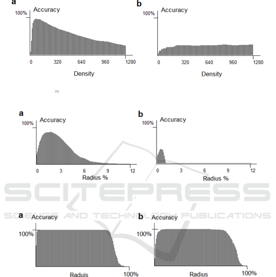
Figure 3: Influence of connection density on pattern recognition accuracy. a, accuracy function at 5%-feature noise on testing
with macrocolumns (
3%R
) and inhibition. b, accuracy function at 5%-feature noise on testing without macrocolumns
and inhibition.
Figure 4: Set recognition accuracy as a function of macrocolumn radius R with and without inhibition of inputs. a, with
inhibition, noise at validation = 5%, best accuracy = 95% at R = 3%. b, no inhibition, noise at testing = 5%, best accuracy =
54% at R = 1%.
Figure 5: Vector recognition accuracy as a function of macrocolumn radius R. a, noise at testing = 50%, accuracy = 100% at
R = 2.3% - 80% of a 256-feature range. b, noise at testing = 100%, accuracy = 100% at R = 10.9% - 59.4% of a 256-feature
range.
Dow-Jones etc., are value indexes. If multiple
values are used as indexes, it becomes possible, for
example, to quickly find a useful pattern in millions
of noisy patterns, instantaneously predict coming
failures of jet engines (Mikhailov, A., Karavay, M.
and Farkhadov, M., 2017), accurately diagnose
diseases with gene expression profiles (Mikhailov,
A. et al., 2023), recognize trademarks images
(Mikhailov, A., Karavay, M., 2023) and so on. Such
numeric inverse indexing can be achieved by
swapping subscripts and values.
6.1 Numeric Inverted Index
Values and their subscript subsets can be flipped as
easily as sides of a coin. Such swap transforms are
a one-to-one correspondence in a sense that values
can be uniquely reconstructed from the subsets of
subscripts and vice versa. These transforms do not
involve any arithmetic operations but just
rearranging of data. This is a reason numeric inverse
indexing can often deliver practically instant
machine learning, because all it takes to train a
On Function of the Cortical Column and Its Significance for Machine Learning
465

connectivity-based system (Figure 1) is to re-
arrange data. Note that all variables in the following
expressions are integers.
Example 1. Given a sequence of values
, 1,..,
n
x n N=
,
xX
where
X
is a set of all distinct values of
n
x
, the
following subsets of subscripts can be constructed:
{ } { : }
xn
n n x x==
,
xX
In mathematics, such subsets are called inverse
images or pre-images, which are referred to in this
paper as inverse patterns. Here, the numeric
inverted index transform is
, 1,..., { } ,
nx
x n N n x X=   
Clearly, each side of the above expression can
be uniquely reconstructed from the other side. The
numeric inverted index algorithm is as follows:
1,..., , { } { }
mm
xx
m N n n m==
with initial conditions:
{ } ,
x
n x X=   
.
Obviously, after executing the algorithm, we have
{ } { } , if
m
k
kmxx
n n x x==
, even though
km
.
The histogram
|{ } |,
xx
h n x X=  
,
represents sizes of subsets indexed by values
Example 2. Given a matrix of
N
distinct rows
1,1 1,
,
,1 ,
()
F
n f N F
N N F
xx
x
xx



=



(1)
where
xX
, the numeric inverted index transform
, , | |
( ) ({ } )
n f N F x f X F
xn


produces an array of sets of row subscripts
1,1 1,
, | |
,1 ,
{ } { }
({ } )
{ } { }
F
x f X F
N N F
nn
n
nn



=



Here, the numeric inverted index algorithm is
given as
, ,
,,
1,..., , 1,..., , { } { }
ff
m f m f
xx
f F m N n n m= = =
with initial conditions:
,
,
{ } , ,
f
mf
x
n m f=  
6.2 Pattern Recognition Task
Given an input pattern
( , 1,..., )
f
x f F==x
and
collection of patterns (1) represented by
N
distinct
rows of features, it is required to find a row that
shares a maximum number of similar features with
the input pattern, that is
1
: ( , ) max ( , )
N
R m R n
n
m H H
=
=x x x x
(2)
A full search would take about
FN
operations
needed to compare the input pattern
x
to
N
template patterns. However, a use of inverse data
representations, that is, numeric inverted indexed
allows reducing the computational complexity on
recognition to
( / )O FN X
.
6.3 Solution to Pattern Recognition
Task
The numeric inverted index transform produces a
matrix of inverse patterns, which allows calculating
Hamming vector similarities
( , )
Rm
H xx
(number of
dimensions with close features) between an input
vector
1
( ,..., )
F
xx=x
and all template vectors
,1 ,
( ,..., )
m m m F
xx=x
,
1,...,mN=
, as samples of the
following index histogram:
,
( , ) |{ : { } }|, 1,...,
f
x x R
R m x f
x x R
f
H f m n m N
+
−
=  =xx
Indeed, the numeric inverse indexing ensures
that
,,
{ } | |
x x R
x f f m f
x x R
f
f
m n x x R
+
−
  − 
Finally, the solution to the pattern recognition
task is a feature vector
m
x
that satisfies (2).
6.4 Set Case
There exist certain differences in processing of
feature vectors and feature sets because the latter
once are unordered, variable size patterns. This is
ICPRAM 2024 - 13th International Conference on Pattern Recognition Applications and Methods
466

the reason the Hamming vector similarity was
replaced with Jaccard similarity measure
( , ) | |/ | |, 1,...,
n n n
S Y X Y X Y X n N==
Here,
, 1,...,{}
nn
NX x n ==
, is a sequence of
enumerated sets and
{}yY =
is an input set. The
inverse sets can be produced by the numeric
inverted index algorithm
{ } { } , , 1,...,
x x m
n n m x X m N=   =
with initial conditions:
{ } ,
xm
m
n x X=   
The Jaccard similarity should be re-written as
||
( , ) , 1,...,
| | | | | |
Rn
nn
Rn
R
YX
S Y X n N
Y Y Y X
==
+−
(3)
Here,
||
Rn
YX
is the random quasi
intersection (Mikhailov, A., Karavay, M., 2023).
Finally, the solution to the feature set recognition
task is the pattern
n
X
that maximizes (3).
7 CONCLUSIONS
1) Cortical column can be mathematically described
as an inverse pattern.
2) A set of cortical columns serves as an inverted
index.
4) Inverted index supports practically instant
learning capabilities even in noisy environments.
3) Increased number of cortical columns enhances
pattern recognition accuracy.
4) Suggested model shows a way of implementing
pattern learning systems that do not use any
arithmetic operations.
REFERENCES
Bastos, A., et al. (2012). Canonical microcircuits for
predictive coding. Neuron. Vol.76 (4): 695–711.
Bledsoe, W., Browing, I. (1959). Pattern recognition and
reading by machine. Proceeding of East.Joint
Comput, Conf., vol.16, 225-232. doi: 10.1145/
1460299. 1460326.
Brin S. and Page L. (1998). The Anatomy of a large-scale
hypotextual web search engine. In Computer
Networks and ISDN System. Vol. 30, Issues 1–7.
Stanford University, Stanford, CA, 94305, USA.
Retrieved from https://doi.org/10.1016/S0169-
7552(98)00110-X
Buxhoeveden, D., Casanova, M. (2002). The minicolumn
hypothesis in neuroscience. Brain.vol.125, 935–951.
Csurska, G. et al. (2004). Visual categorization with bags
of keypoints. Proceedings of ECCV International
Workshop on Statistical Learning in Computer
Vision.
DeFelipe, J. (2012). The neocortical column. Frontiers in
Neuroanatomy.vol. 6: 5.
Harris, Z. (1954). Distributional Structure. Word. 20
(213). 146-162.
Horton, J., Adams, D. (2005). The cortical column: a
structure without a function. Philos. Trans. R. Soc.
Lond. B Biol. Sci. vol. 360 (1456): 837–862.
LeDoux, J. (2002). Synaptic self. Viking Penguin.
Marcus, G., Marblestone, A., Dean, T. (2014).The atoms
of neural computation. Science. vol. 346, ISSUE
6209, 551-552.
Mikhailov, A.,Karavay, M., Farkhadov M. ( 2017).
Inverse Sets in Big Data Processing. In Proceedings
of the 11th IEEE International Conference on
Application of Information and Communication
Technologies (AICT2017, Moscow). М.: IEEE, vol. 1
https://www.researchgate.net/publication/32130917
7Inverse_Sets_in_Big_Data_Processing.
Mikhailov, A., Karavay, M. (2023). Random Quasi
Intersection with Applications to Instant Machine
Learning. In Proceedings of the 12
th
International
Conference of Pattern Recognition Applications and
Methods. ISBN 978-989-758-626-2, ISSN 2184-
4313, pp. 222-228.
Mikhailov, A. et al. (2023). Machine Learning for
Diagnosis of Deseases with complete Gene
Expression Profile. Automation and Remote Control,
vol. 84, No7, pp. 727-733.
Mountcastle, V. (1957). Modality and topographic
properties of single neurons of cat's somatic sensory
cortex. J. of Neurophysiology. vol,20 (4): 408–434.
Mountcastle, V. (1997). The columnar organization of the
neocortex. Brain. vol.120 (4): 701–722.
Semendeferi, K. et al. (2011). Spatial organization of
neurons in the frontal pole sets humans apart from
great apes. Cerebral Cortex. vol. 21 Issue 7, 1485-
1497
Sivic, J., Zisserman, A. (2009). Efficient visual search of
videos cast as text retrieval. In IEEE Transactions
on Pattern Analysis and Machine Intelligence. vol.
31, Issue: 4. doi: 10.1109/TPAMI.2008.111
Squire, L. (2013). Fundamental Neuroscience (4
th
ed.),
Academic Press.
Tsunoda, K. et al. (2001). Complex objects are
represented in macaque inferotemporal cortex by the
combination of feature columns. Nat. Neurosci. vol. 4
(8): 832–838.
Wilson, D. (2008). How do we remember smells for so
long if olfactory sensory neurons only survive for
about 60 days. Scientific American. vol.298, No 1, 91.
On Function of the Cortical Column and Its Significance for Machine Learning
467

APPENDIX
This section provides details of computer
experiments described in Section 5.
Experiment 1: The collection of 1280 random
patterns, where each pattern was represented by a
variable length feature set, was created T times.
Each time, the system’s memory was reset and the
system re-trained with the next 1280-pattern
collection by using the numeric inverted index
transform (Section 6.1). The number of columns in
the region was C = 256. In accordance with the
connectivity equation,
/D FN C=
, the connection
density kept on increasing at each training session
by incrementing the average pattern size:
F
=1%,
2%,…,100%. The random feature values of each
pattern were uniformly distributed in the interval [0,
C-1]. The random lengths of patterns were normally
distributed in the interval
[ 0.05 , 0.05 ]F C F C−+
.
On each testing run, each feature x from the current
pattern collection was distorted by
5%  =
random
noise, that is,
(1 )xx  =
. The experiment was
conducted twice. For the first training/testing batch,
the radius was set to R = 3% of the value of C,
leading up to almost a 100% accuracy. For the
second batch, the radius was set to 0, resulting in a
poor performance.
Experiment 2: The collection of 1280 random
patterns, where each pattern was represented by a
variable length feature set, was created only one
time. The average pattern size was set to 64 features.
As in experiment 1, the random feature values of
each pattern were uniformly distributed in the
interval
[0, -1]C
. The random lengths of each
pattern were normally distributed in the interval
[ 0.05 , 0.05 ]F C F C−+
.
For a testing, each feature x from the training pattern
collection was distorted by
5%  =
random noise.
Unlike experiment 1, the macrocolumn radius kept
on increasing at each testing run as R = 1%, 2%, …,
32% of C. Although training was conducted only
once, the 32 testing runs were conducted twice.
Whereas the first testing batch involved a use of
inhibition, the second testing batch was inhibition
free, resulting in a poor performance.
Experiment 3: In this experiment, 1280 vectors
in
F
- dimensional space (
F
= 128) were employed
to train the system using the numeric inverted index
algorithm (Section 6.1). The uniformly distributed
random components of vectors ranged from 0 to
255. The test set contained the same vectors that
were engineered from training set by way of
distorting original vectors’ components x by
50%  =
noise of the value of the corresponding
component. The pattern size was fixed at
F
= 128.
All 1280 test vectors were submitted for
recognition. The resulting accuracy function
achieves a 100%-level for a wide range of R. Note
that in the vector case, inhibition policy is not
needed.
ICPRAM 2024 - 13th International Conference on Pattern Recognition Applications and Methods
468