Ki67 Expression Classification from HE Images with Semi-Automated
Computer-Generated Annotations
Dominika Petr
´
ıkov
´
a
1 a
, Ivan Cimr
´
ak
1 b
, Katar
´
ına Tobi
´
a
ˇ
sov
´
a
2
and Luk
´
a
ˇ
s Plank
2 c
1
Cell-in-fluid Biomedical Modelling & Computations Group, Faculty of Management Science and Informatics,
University of
ˇ
Zilina, Slovak Republic
2
Department of Pathology, Jessenius Medical Faculty of Comenius University and University Hospital, Martin,
Slovak Republic
Keywords:
Ki67 Index, Hematoxylin-And-Eosin, Classification, Neural Networks, Digital Pathology.
Abstract:
Ki67 protein plays crucial role in cell proliferation and it is considered a good marker for determining the cell
growth. In histopathology, it is often assessed by immunohistochemistry (IHC) staining. Even though IHC is
considered common practice in clinical diagnosis, it has several limitations such as variability and subjectivity.
Meaning interpretation of IHC can be subjective and vary between individuals. Moreover, quantification can
be challenging as well as it is cost and time consuming. Therefore neural network models hold promise for
improving this area, however they require a large amount of high quality annotated dataset, which is time-
consuming and laborious work for experts. In the paper, we employed the proposed semi-automated approach
of generating Ki67 score from pairs of hematoxylin and eosin (HE) and IHC slides, which aims to minimize
expert assistance. The approach consists of image analysis methods such as clustering optimization for tissue
registration. Using a sample of 84 pairs of whole slide images of seminomas tissue stained by HE and IHC,
we generated dataset containing approximately 30 thousand labeled patches. On the HE patches annotated by
proposed approach, we executed several experiments on fine-tuning neural networks model to predict Ki67
score from HE images.
1 INTRODUCTION
Digital pathology and image analysis have important
roles in diagnostic of many diseases including cancer.
It requires digital scans of high quality tissue samples
in high-resolutions generated by digital scanners as
whole slide images (WSIs). Development of digital
scanners has enabled generation of large amounts of
histopathology data, which can be processed by ma-
chine learning algorithms for many tasks including
classification of the tisue specimen (Hamilton et al.,
2014; Pantanowitz, 2010).
Histopathological analysis of all tissues, includ-
ing malignant tumours, is performed on 3-4µm thick
sections of formalin-fixed paraffin embedded (FFPE)
sections stained first with hematoxylin and eosin.
This staining enables basic evaluation of morphology
of malignant tumour, including parameters such as
mitotic activity, invasion of adjacent structures, and
a
https://orcid.org/0000-0001-8309-1849
b
https://orcid.org/0000-0002-0389-7891
c
https://orcid.org/0000-0002-1153-1160
grading. Grading corresponds to the degree of re-
semblance of tumour cells to the original healthy tis-
sue. Well-differentiated tumours (G1, G2) in gen-
eral have a more favourable outcome, poorly dif-
ferentiated tumours (G3 or G4 resp.) behave more
agressively and have worse prognosis. Certain cate-
gories of tumours, such as neuroendocrine neoplasias
of gastroenteropancreatobiliary and respiratory tract,
require immunohistochemical analysis of tumor pro-
liferation activity as a part of their grading. This
analysis uses the IHC antibody against the so-called
proliferation factor (Ki67), a nuclear protein associ-
ated with ribosomal RNA transcription expressed dur-
ing interphase of proliferating cells (Bullwinkel et al.,
2006). Testicular seminoma is the most common tes-
ticular germ cell tumour and the most common malig-
nant tumour among young men (Krag Jacobsen et al.,
1984). Prognosis depends on clinical stage at the time
of diagnosis, tumour size, rete testis invasion and vas-
cular invasion. Proliferation index in seminoma tends
to exceed 50% (Rabes et al., 1985), but lower values
(below 20%) can be found as well. High prolifera-
536
Petríková, D., Cimrák, I., Tobiášová, K. and Plank, L.
Ki67 Expression Classification from HE Images with Semi-Automated Computer-Generated Annotations.
DOI: 10.5220/0012535900003657
Paper published under CC license (CC BY-NC-ND 4.0)
In Proceedings of the 17th International Joint Conference on Biomedical Engineering Systems and Technologies (BIOSTEC 2024) - Volume 1, pages 536-544
ISBN: 978-989-758-688-0; ISSN: 2184-4305
Proceedings Copyright © 2024 by SCITEPRESS – Science and Technology Publications, Lda.

tion index in seminoma does not correlate with clin-
ical stage and presence of distant metastases (Galle-
gos et al., 2011), however, one study detected a sig-
nificant inverse association with rete testis invasion
and the expression of Ki67 in more than 50% of cells
(Lourenc¸o et al., 2022). In order to initiate machine
based learning on HE and Ki67 stained slides contain-
ing samples of testicular seminoma, we established
three different thresholds for Ki67 expression: below
20%, 20-50% and above 50%.
In practice, multiple IHC and HE staining is per-
formed on adjacent tissue sections. This allows
pathologists to examine different tissue characteris-
tics in the same area on adjacent slides. Although
adjacent regions have similar spatial characteristics,
they are not identical to other specimens. Moreover,
these can still be rotated and displaced, so it is very
important to align these differently stained histolog-
ical scans together in order to use machine learning
analysis.
Training a deep neural network requires a large
amount of high quality annotated images as a train-
ing dataset. Since the WSIs are too large to be pro-
cessed as a whole by the neural network, they need to
be divided into smaller images, called patches. Con-
sequently, for patch annotation we distinguish several
approaches such as whole slide-level, region-level,
cell-level. The difficulty of evaluating patches among
these approaches increases rapidly in terms of the ef-
fort required for creation as well as the expertise of
the evaluator.
Whole slide annotations are also referred to as
weak annotations because all patches from a single
slide share a common annotation, regardless of the
fact that the tissue on them may be heterogeneous.
Such a dataset may be easier to obtain, but its use is
quite limited and requires a special approach called
weakly-supervised learning. For example, (Li et al.,
2021) used Multiple instance learning for prostate
biopsy WSI classification and weakly-supervised tu-
mor region detection.
In order to train a machine learning classifier for
cell-level annotation, the images must first be anno-
tated with the boundaries of each cell and its sub-
types. The cell-level annotation process requires a
huge manual effort, which can be facilitated by using
cell segmentation followed by region-level annotation
to capture cell-level features, such as presence of tu-
mor infiltrating lymphocytes (Saltz et al., 2018). The
use of region-level annotations assumes that the cells
in the annotated region have the same cell types (Lee
et al., 2021).
Region-level annotations require additional input
from experts. For instance, pathologists have to local-
ize and annotate all pixels or cells in WSI by contour-
ing the whole tumor. Although creating region-level
(or patch-level) annotations is more challenging, it is
reasonable and we will discuss this approach more in
this paper. In (Yang et al., 2021), EfficientNet and
ResNet (Residual Net) were employed to carry out
patch-level classification of lung lesions into 6 types.
To aggregate patch predictions into slide-level classi-
fication two methods were compared: majority voting
and mean pooling. Similar approach was used in (Luo
et al., 2022) to perform the binary subtype classifica-
tion of eyelid carcinoma. Authors used DenseNet-161
to make predictions for every patch in WSI and then
used a patch voting strategy to decide the WSI sub-
type.
Obtaining IHC staining is a standard procedure
in clinical practice to determine tissue molecular in-
formation, however it has several limitations. IHC
is time-consuming, expensive, and highly dependent
on tissue handling protocols because the output is
expressed as stain intensity or presence/absence of
stain or the percentage of cells that achieve detectable
stain intensity (Naik et al., 2020). Many recent stud-
ies showed that there exists correlation between HE
and IHC stained slides from the same region (Naik
et al., 2020; Seegerer et al., 2020; Rawat et al., 2020).
Therefore it should be possible to predict expression
of specific proteins directly from HE slides. The prob-
lem of prediction Ki67 cell positivity from HE im-
ages was addressed in (Liu et al., 2020). Authors
fine-tuned ResNet18 at the cell-level annotated HE
images.To obtain annotated cell patches point label
approach on homogeneous Ki67 positive or negative
regions was employed. Subsequently, trained CNN
was transformed into fully convolutional network, so
it was able to handle WSI as input and prodcuse
heatmap of Ki67 concentration on the whole slide
image as output. In (Shovon et al., 2022), modified
Xception network was proposed to classify HE im-
ages into four categories based on Human epidermal
growth factor receptor 2 (HER2) positivity.
Contents of This Work
The aim of this work is to train neural network model
for classification of Ki67 protein expression from HE
images. First, we describe the proposed method of
semi automated dataset creation and then show exper-
iments made in training several neural network mod-
els for classification.
The dataset consists of individually labeled HE
patches representing the amount of Ki67 protein ex-
pressed on that patch. These patches were cut from
HE whole slide images and annotated based on Ki67
Ki67 Expression Classification from HE Images with Semi-Automated Computer-Generated Annotations
537

expression on IHC whole slide images of the same
tissue. For the purpose of training the neural net-
work, HE and IHC staining was used on adjacent tis-
sue sections to make the tissue as identical as possible.
Hence we assume that based on spatial proximity of
the physical slides from which HE and Ki67 images
were obtained, a patch from the HE whole slide im-
age can be labelled by the patch from the Ki67 whole
slide image from the same location.
In Section 2 we describe laboratory and mathe-
matical methods. First we describe laboratory proto-
cols for tissue sample and image acquisition. Then
we present data preprocessing and steps leading to
creating annotations. Further we present optimization
method used to align Ki67 and HE images. Finally,
the end of the section is devoted to introduction of ma-
chine learning methods, specifically neural networks,
for prediction tasks with image data.
In Section 3 we provided details of the data an-
notation and dataset creation process. This includes
results of the enhanced Ki67 and HE images regis-
tration through optimization method with defined key
points. Further we show details of color clustering
and modifications needed. Finally, we present experi-
ment results of a neural networks classification of HE
patches into two Ki67 labels.
2 METHODS
2.1 Image Acquisition
84 samples of testicular seminoma were sectioned
into 3-4mm thick parallel FFPE sections. HE
staining was performed on Tissue-Tek Prisma®
Plus Automated Slide stainer (Sakura Finetek Japan
Co.,Ltd.) on deparaffinized sections with Weigert
hematoxylin, which were then washed and differ-
entiated with low pH alcohol, washed and put into
eosin, dehydrated, cleared with carboxylole and
xylene and finished slides were coverslipped with
Tissue-Tek Film® Automated Coverslipper (Sakura
Finetek Japan Co.,Ltd.). Immunohistochemical anal-
ysis was performed with the monoclonal mouse an-
tibody clone MIB-1 (FLEX, Dako), on automatized
platform PTLink (Dako, Denmark A/S). Visualization
was performed using EnVision FLEX/HRP (Dako),
DAB (EnVision FLEX, Dako) and cotrast hema-
toxylin staining. HE and Ki67 whole slides from
the same case were ordered successively, anonymized
and scanned in 3D Histech PANORAMATIC© 250
Flash III 3.0.3, in BrightField Default mode. WSIs
were annotated for areas of tumour and non-tumorous
tissue and for the so-called ”hot spots” with the high-
est density of positive IHC reaction.
2.2 Data Preprocessing
In order to use image analysis methods on the data,
we first had to convert it from the original mrxs for-
mat to png using the OpenSlide library in python.
The original format can store images of samples from
glass slides at multiple levels with different resolu-
tions. Our scans contain images in 8 levels. Due
to the memory requirements of the highest resolution
images, we decided to process the images at a lower
level with second highest resolution. They are still
detailed enough without information loss while not
causing a memory problem. HE scans contained two
tissue sections, therefor we extracted super patches
containing only one tissue from the original scans.
The same procedure was also applied to IHC scans,
which significantly reduced the size of the resulting
png images.
Obtained data do not contain any additional in-
formation about Ki67 expression that could be used
as a label apart from the pairs of scans themselves.
Therefore, we devised improved method based on
(Petr
´
ıkov
´
a et al., 2023) to estimate the ratio of positive
cells to all cells on patches from Ki67 scans, which
we then use as annotations for HE patches. Proposed
method consists of three steps: slides registration, col-
ors clustering, quantification of Ki67 score.
Each tissue sample is rotated differently on the
slide. First, it was necessary to align the images so
that tissues from the same area are in the same posi-
tion. We defined alignment as rotation and shift. In
our improved method, we tried a different approach
of registration, which will be described in the next
subsection.
After slides alignment, K-means clustering is ap-
plied to Ki67 stained image to obtain main colors
of the tissue. These colors are then divided into
three categories: positive cells (brown colors), nega-
tive cells (blue colors) and background (white colors).
Next, the whole image is recolored according to clus-
tering result. From obtained recolored Ki67 image it
is possible to estimate Ki67 score as:
ratio =
brownpixels
brownpixels +bluepixels
(1)
2.3 BFGS Optimization
To align the pairs of scans, we needed to find trans-
formation parameters to rotate and shift the images
using the defined key points.That is, for pairs of key
points from the Ki67 scan and the HE scan that corre-
sponded to the same location on the tissue, we needed
BIOINFORMATICS 2024 - 15th International Conference on Bioinformatics Models, Methods and Algorithms
538

to optimize two transformation parameters.
The BFGS method (named for its discoverers
Broyden, Fletcher, Goldfarb and Shanno) is the most
popular second order optimization algorithm belong-
ing to class of quasi-Newton methods. These meth-
ods approximate the second derivative also called the
Hessian and the inverse of the Hessian matrix using
the gradient, meaning that the Hessian and its in-
verse do not need to be available or calculated pre-
cisely for each step of the algorithm. By measuring
the changes in gradients, quasi-Newton methods con-
struct a model of the objective function that can pro-
duce superlinear convergence. They require only gra-
dient of the objective function at each iteration, which
makes them sometimes more efficient than Newton’s
method since second derivatives are not required. In
Newton’s methods Hessian can be used to determine
both the direction and the step size to move, so the
input parameters change in order to minimize the ob-
jective function. In BFGS, the direction of move can
be expressed from approximation of inverse of Hes-
sian like:
p
k
= −H
k
∇ f
k
. (2)
However it is not possible to use approximation of
the Hessian inverse to determine step size α
k
. The al-
gorithm addresses this by using a line search in the
chosen direction to determine how far to move in that
direction that satisfies Wolfe conditions. From direc-
tion p
k
and step size α
k
new iterate can be computed
as:
x
k+1
= x
k
+ α
k
p
k
, (3)
. To simplify the formula for inverse Hessian approx-
imation, we can define the vectors s
k
and y
k
as:
s
k
= x
k+1
− x
k
, (4)
y
k
= ∇ f
k+1
− ∇ f
k
. (5)
The solution of inverse Hessian approximation is then
given by
H
k+1
= (I − ρ
k
s
k
y
T
k
)H
k
(I − ρ
k
y
k
s
T
k
) + ρ
k
s
k
s
T
k
, (6)
with
ρ
k
=
1
y
T
k
s
k
. (7)
Given starting point x
0
, convergence tolerance ε >
0 and inverse Hessian approximation H
0
, the BFGS
algorithm can be summarized as follows:
1. set k = 0
2. while ∥∇ f
k
∥ > ε;
3. compute search direction p
k
and step size α
k
4. set x
k+1
according to (5)
5. compute H
k+1
by means of (6)
6. set k = k +1
7. end (while).
Before running the algorithm, it is necessary to found
initial approximation H
0
. There is no general pro-
cedure on how to set the initial approximation. It is
possible to set it as an identity matrix or its multiple,
or to use problem specific information (Nocedal and
Wright, 2006; Griva et al., 2008).
2.4 Convolutional Neural Networks
Ever since it was possible to scan and load images
into computers, researchers were trying to develop au-
tomated system for image analysis. One of the most
popular machine learning approaches used in medical
image analysis are supervised techniques using exam-
ple data with corresponding labels. The basis of these
algorithms is to learn connections and patterns in data
itself to find a model for mapping inputs to outputs.
Creating model involves finding the best parameters
that can be used to predict outputs for inputs based on
a defined loss function (Jordan and Mitchell, 2015;
Litjens et al., 2017).
Neural networks form the basis of the most deep
learning algorithms. They consist of neurons, inter-
connected units, with activation and parameters orga-
nized into multiple layers. By now, there are several
types of neural networks adapted to certain tasks.
One of the most widely used is the convolutional
neural networks (CNNs). It was primarily introduced
for processing of visual data like images and videos,
although, they can be extremely useful for almost
any type of data (Litjens et al., 2017; Wang et al.,
2018). CNNs consist of three types of layers: con-
volutional layers, pooling layers, and fully connected
layers. The most significant component of the CNN
architecture is the convolutional layer with its filters,
also called kernels. Kernels are represented as a grid
of discrete values referred to as kernel weights and
contribute to the convolution operation. In particular,
these kernel weights, adjusted during training, slide
over the entire image horizontally and vertically to
obtain a feature maps. The dimensionality of gener-
ated feature maps is reduces by pooling layers. Con-
volutional layers together with pooling layers build
pipeline called feture extraction, which detects local
features in the input data. Similar to classical multi-
layer perceptron networks, the lower layers of CNNs
learn basic features and kernels of deeper layers learn
more and more complex features. At the end of CNN
architecture, there are fully-connected layers, which
combine local features extracted by the previous lay-
ers to obtain global features, and perform the final
classification task (Ahmad et al., 2019; O’Shea and
Ki67 Expression Classification from HE Images with Semi-Automated Computer-Generated Annotations
539

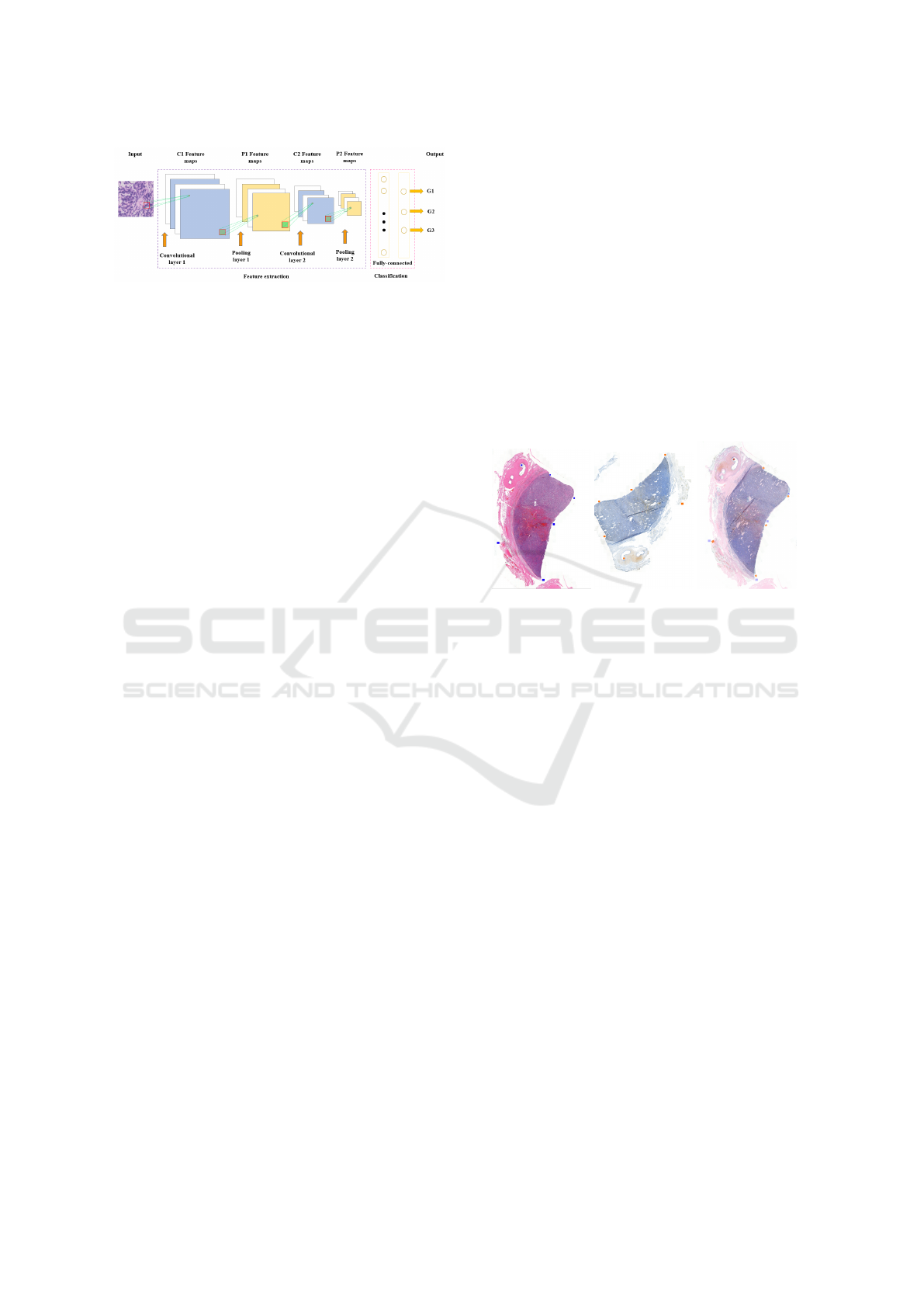
Figure 1: Convolutional neural network architecture.
Nash, 2015; Alzubaidi et al., 2021). Typical CNN ar-
chitecture is displayed in Figure 1
Critical factor in improving the performance of
different applications is model architecture. From
first CNN model, various modifications have been
achieved. Key upgrade in performance of CNNs oc-
curred due to the processing-unit reorganization, as
well as the development of novel blocks. The most
novel developments in CNN architectures were per-
formed on the use of network depth (Alzubaidi et al.,
2021). To date, there are several proven architec-
tures that are frequently used in a wide range of do-
mains. These architectures can be trained with ini-
tialized weights from scratch or fine tuned from pre-
trained weights on known large datasets such as Im-
ageNet. Examples of such architectures are VGG
(Visual Geometry Group), ResNet, DenseNet or nets
from the Inception family.
3 RESULTS
3.1 HE - Ki67 Registration
For this research, we were able to produce 84 pairs
of HE and Ki67 scans of tissue specimens of semi-
nomas (testicular tumors). Before the actual opti-
mization of the rotation and displacement parame-
ters, it was necessary to define key points for each
pair of scans and mark them on the images. For this,
we used the SlideViewer software, which can display
multiple scans simultaneously and create annotations.
Each key point was created as a square annotation,
with five key points defined for a single pair of scans.
In addition to these, on each slide we marked with
a square annotation the area where the tissue is lo-
cated and which will be further processed. This al-
lowed us to make tissue bounding box cutouts from
the WSIs, which significantly reduced the size of the
images. The adjacent image pairs were adjusted to
have the same dimensions by adding white pixels to
the smaller one. The existing annotations were ex-
ported to xml files via SlideMaster and converted to
key point coordinates, taking the center of the anno-
tation as the coordinate. The objective function was
the sum of the distances of each pair of the original
HE coordinates and the calculated new IHCs. The
new coordinates were calculated from the parameters
of the current iteration using matrix operations for in-
plane translation and rotation. The resulting rotation
was applied to the IHC image, performing it around
the center with pixel replenishment. We added white
pixels to the HE image to make it the same size and
centered it. We then shifted the original HE tissue im-
age by the calculated parameter in the negative direc-
tion, resulting in an aligned pair of images with the
same dimensions. An illustration of the transforma-
tion performed along with the key points highlighted
is shown in Figure 2. With this procedure, we were
able to automatically align 79 pairs of scans.
Figure 2: Registration example, on the left original HE tis-
sue with highlighted keypoints (blue points), in the middle
original IHC tissue with highlighted keypoints (red points),
on the right overlay of HE tissue with registered IHC tissue.
3.2 Construction of Dataset
The next step in annotation extraction was to apply
the Kmeans clustering algorithm to the IHC images
to obtain the dominant colors. Due to the size of the
images we were working with, it was not possible to
apply clustering to the whole image at once, but had
to be divided into smaller parts. However, even on
the smaller parts, the algorithm took several hours to
compute, significantly increasing the number of hours
spent per image. Therefore, we decided not to do
clustering on all parts of the image, but to choose one
region that is quite representative and contains a wide
range of all colors. Subsequently, all pixels from the
image were assigned to one of the obtained centroids.
These centroids had to be categorized into one of
three classes: Ki67 positive cell (brown), Ki67 neg-
ative cell (blue), and background (white) based on
which objects in the scan corresponded to each color.
Even though we increased the number of clusters k
from the original 6 to 12, for some scans there were
no brown shades among the dominant colors. This
is due to the general low Ki67-positivity of the tissue
on our scans. Applying such centroids would have
suppressed the low number of Ki67-positive cells to
BIOINFORMATICS 2024 - 15th International Conference on Bioinformatics Models, Methods and Algorithms
540

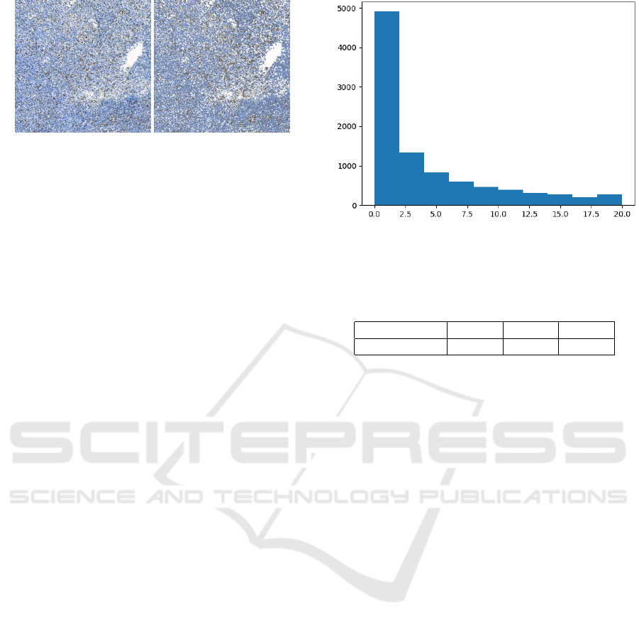
Figure 3: Comparison of original image and recolored one
after clustering.
zero, thus creating incorrect, misleading annotations.
In this case, we used centroids from another image
that had a similar color spectrum and its centroids
contained brown. An example of a comparison be-
tween the original IHC tissue and an image recolored
into 3 colors based on centroids is shown in Figure 3.
The recolored image served as the basis for the eval-
uation of Ki67 patch scores according to the formula
(1).
HE patches with annotation estimated from
patches of the redrawn image were generated with a
size of 224x224 pixels and only under the condition
that the pixel ratio in the white shades correspond-
ing to the background was below a certain thresh-
old. For HE patches we set the threshold to 40%, for
Ki67 patches the value was higher, up to 60%. How-
ever, even among these patches, there were still some
patches that did not contain cells, in case the back-
ground color was darker than our thresholds. There-
fore, it was still necessary to additionally remove the
incorrect data. From the counts of generated patches
mentioned above, it is clear that our dataset is heavily
imbalanced, which may cause problems during model
training. Due to the high amount of data, we de-
cided to balance the dataset using an undersampling
method, in which the classes with higher data counts
are reduced in the process. We randomly selected ap-
proximately 10,000 patches from the below 20% and
20-50% categories to be used as part of the dataset.
The resulting dataset thus had the following distri-
bution: 9632 patches of below 20%, 9419 patches of
20-50% and 10 576 patches of above 50%. The exam-
ple of detailed distribution of the first class in dataset
is displayed in the histogram Figure 4.
3.3 Training Neural Networks
For the purpose of validation, we split the dataset into
training and validation sets in a 9:1 ratio. In addition
to data balancing, we also used horizontal and verti-
cal flip data augmentation for training. Moreover, the
data were normalized before entering into the model.
In all experiments, we trained the ResNet archi-
Figure 4: Dataset distribution of class below 20%, on x axis,
there is Ki67 ratio of patches grouped into bins by 2%, y
axis represents counts of patches.
Table 1: Accuracy of ResNet18 model with different learn-
ing rates.
Learning rate 0.1 0.01 0.001
Accuracy 0,7785 0,7674 0,7471
tecture with pre-trained weights on ImageNet namely
ResNet50 and smaller ResNet18. Since preliminary
results showed that ResNet18 exhibited higher accu-
racy on the validation set, we decided to further inves-
tigate the best hyperparameter setting on this archi-
tecture only. We replaced the classification part of the
original architecture with two fully-connected layers
with 512 and 3 neurons respectively. A dropout with a
value of 0.2 was used on the penultimate layer. In ad-
dition to the network depth itself, we also compared
two types of optimizer: Adam and SGD (Stochastic
gradient descent). In Figure 5 we can see example
plots of the evolution of the loss on the validation and
training sets for both optimizers. From the compar-
ison, we can observe that the loss progression with
SGD was more stable, so we used only the latter in
the following experiments. All models were trained
for 50 epochs with a batch size of 64, unless other-
wise stated. Below we describe the most important
one.
In Table 1 are the results of the models for differ-
ent learning rates. Although in this case 0.1 seemed
to be the best choice, in later experiments 0.01 proved
to be a better choice.
Because of the present overfitting, we tried adding
regularization and momentum in the next experiment
(Table 2). Among several possibilities, 0.0001 proved
to be the best value for weight decay. Larger values
caused the model to be underfitted adn lower values
failed to eliminate the overfitting problem. We tried
to increase the accuracy by changing the batch size,
but as we can see in the Table 3 the chosen batch size
Ki67 Expression Classification from HE Images with Semi-Automated Computer-Generated Annotations
541

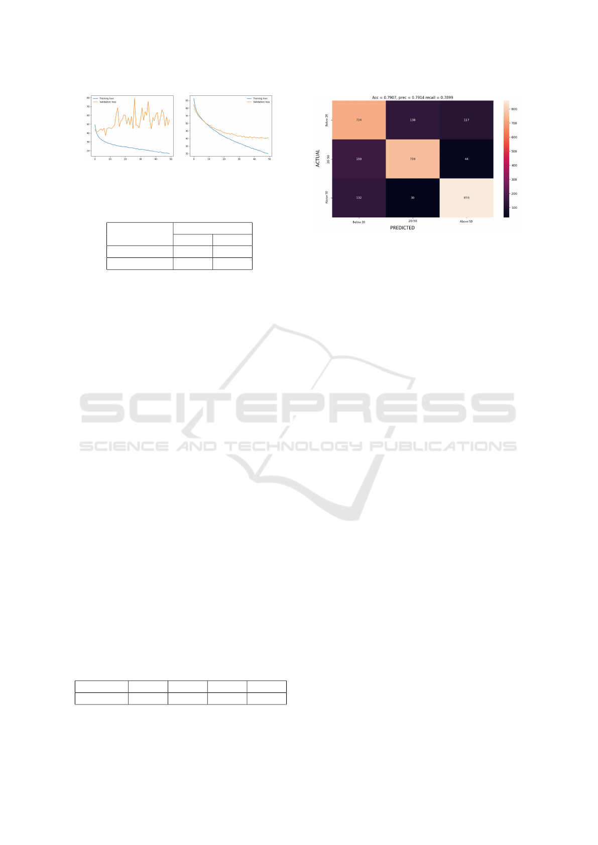
Figure 5: Comparison of ResNet18 model loss function
with optimizer Adam (left) and SGD (right).
Table 2: Accuracy of ResNet18 model with different pa-
rameters of regularization and momentum.
Weight decay
Momentum
None 0.9
None 0,7539 0,7768
0.0001 0,7391 0,7907
64 achieved the highest accuracy.
The highest accuracy achieved on the validation
set was 0.79, which is quite low. From the confusion
matrix of the best model on the validation set shown
in Figure 6, it is clear that it is most difficult for the
model to distinguish patches from the category be-
low 20%. But it is able to distinguish between the
other two categories quite well. To test this hypoth-
esis, we tried to train a binary model distinguishing
between patches from the 20-50% and above 60% cat-
egory. We purposely omitted the interval between 50
and 60% to test what accuracy it achieves on a sim-
pler task. In this case, the best model achieved 0.8595
accuracy, and after adding the omitted interval to the
new model, the accuracy only dropped to 0.8484.
Even though the model achieves higher accuracy
for binary classification, neural networks have the po-
tential to achieve better results. Therefore, we pro-
posed possible reasons and improvements for the fu-
ture, mainly related to dataset modification. As a first
step, we need to verify that our proposed annotation
method is correct on this data as well, since it differs
from the data on which it was originally validated.
Another problem could be that patches are generated
from the whole slide and although we tried to auto-
matically discard those containing a small amount of
tissue, we could not remove all of them. In addition,
there are also parts of the tissue where there are few
cells or the tissue is somehow damaged. These ar-
eas would need to be discarded or regions of inter-
est marked on the slides from which to determine the
score.
Table 3: Accuracy of ResNet18 model with different batch
size.
Batch size 8 32 64 128
Accuracy 0,7417 0,7758 0,7907 0,7812
Figure 6: Confusion matrix of the best multiclass ResNet18
model on validation set, on x axis predicted classes, on y
axis actual (ground truth) classes.
4 CONCLUSIONS
In this paper, we attempted to develop a neural net-
work model for classifying Ki67 scores from HE im-
ages using a semi-automated annotation generation
method. We proposed an improvement to the pre-
vious annotation extraction method. In contrast to
(Petr
´
ıkov
´
a et al., 2023), we used manually defined
keypoint pairs for registration. Among these pairs,
we found the optimal transformation parameters us-
ing the BFGS optimization method. With this im-
provement, we were able to successfully register most
of the scan pairs. Then, with the labeled patches, we
tried to train several models on multi-class classifica-
tion as well as on the binary classification task.
Nevertheless, this work has several limitations in-
volving the lower accuracy of the classification mod-
els on the validation set. We have proposed several
reasons for this and possible solutions for the future
concerning the modification of the training dataset.
Regardless of this, it is clear from the results that neu-
ral networks have the potential to estimate IHC fea-
tures directly from HE stained tissue. However, this
is only the beginning of our experiments with train-
ing neural network models. There are still challenges,
like:
1. The accuracy of the workflow for generating Ki67
score annotations on this data is unknown. Since
we do not have any annotations on our data, we
are not able to judge whether our approach is ac-
curate or has some bias. In the future, our goal
is to use medical software to obtain estimates of
Ki67 scores on some scans and compare them
with the estimates generated by semi-automated
method.
2. Proliferation activity needs to be evaluated within
areas of the highest density of positive staining
BIOINFORMATICS 2024 - 15th International Conference on Bioinformatics Models, Methods and Algorithms
542

(so-called hot spots) on the minimal number of
500 tumour cells, ideally more than 1000. Other
populations present in tumour, such as stromal
tissue and tumour infiltrating immune cells, also
stain with Ki67 and can skew the result. These
cells are not included into the tumor proliferation
activity evaluation. Currently available machine
based learning programs allow training of recog-
nition of tumour and non-tumour cells in order to
maintain a highly reliable result comparable with
manual counting of a trained pathologist. In or-
der for the model’s predictions to be closer to the
pathologists’ procedure, it will be necessary to
train and evaluate the model only on patches from
tumor region.
Our future research will mainly focus on the follow-
ing aspects. First, improve the accuracy of the models
by conducting a wider range of experiments. Part of
this step will also be the verification of the annota-
tions generating method and a closer examination of
the data that are incorrectly classified by the model.
Second, employ explanation methods on neural net-
works, so we will gain better knowledge about the ar-
eas according to which the model makes decisions.
ACKNOWLEDGEMENTS
This research was supported by the Ministry of Ed-
ucation, Science, Research and Sport of the Slovak
Republic under the contract No. VEGA 1/0369/22.
REFERENCES
Ahmad, J., Farman, H., and Jan, Z. (2019). Deep Learn-
ing Methods and Applications, pages 31–42. Springer
Singapore, Singapore.
Alzubaidi, L., Zhang, J., Humaidi, A. J., Al-Dujaili, A.,
Duan, Y., Al-Shamma, O., Santamar
´
ıa, J., Fadhel,
M. A., Al-Amidie, M., and Farhan, L. (2021). Review
of deep learning: concepts, cnn architectures, chal-
lenges, applications, future directions. Journal of Big
Data, 8(1):53.
Bullwinkel, J., Baron-L
¨
uhr, B., L
¨
udemann, A., Wohlen-
berg, C., Gerdes, J., and Scholzen, T. (2006). Ki-67
protein is associated with ribosomal RNA transcrip-
tion in quiescent and proliferating cells. J. Cell. Phys-
iol., 206(3):624–635.
Gallegos, I., Valdevenito, J. P., Miranda, R., and Fernan-
dez, C. (2011). Immunohistochemistry expression of
p53, ki67, CD30, and CD117 and presence of clinical
metastasis at diagnosis of testicular seminoma. Appl.
Immunohistochem. Mol. Morphol., 19(2):147–152.
Griva, I., Nash, S. G., and Sofer, A. (2008). Linear and
Nonlinear Optimization (2. ed.). SIAM.
Hamilton, P. W., Bankhead, P., Wang, Y., Hutchinson, R.,
Kieran, D., McArt, D. G., James, J., and Salto-Tellez,
M. (2014). Digital pathology and image analysis in
tissue biomarker research. Methods, 70(1):59–73. Ad-
vancing the boundaries of molecular cellular pathol-
ogy.
Jordan, M. I. and Mitchell, T. M. (2015). Machine learn-
ing: Trends, perspectives, and prospects. Science,
349(6245):255–260.
Krag Jacobsen, G., Barlebo, H., Olsen, J., Schultz, H. P.,
Starklint, H., Søgaard, H., and Vaeth, M. (1984).
Testicular germ cell tumours in denmark 1976-1980.
pathology of 1058 consecutive cases. Acta Radiol.
Oncol., 23(4):239–247.
Lee, K., Lockhart, J. H., Xie, M., Chaudhary, R., Slebos,
R. J. C., Flores, E. R., Chung, C. H., and Tan, A. C.
(2021). Deep learning of histopathology images at the
single cell level. Frontiers in Artificial Intelligence, 4.
Li, J., Li, W., Sisk, A., Ye, H., Wallace, W. D., Speier, W.,
and Arnold, C. W. (2021). A multi-resolution model
for histopathology image classification and localiza-
tion with multiple instance learning. Computers in Bi-
ology and Medicine, 131:104253.
Litjens, G., Kooi, T., Bejnordi, B. E., Setio, A. A. A.,
Ciompi, F., Ghafoorian, M., van der Laak, J. A., van
Ginneken, B., and S
´
anchez, C. I. (2017). A survey
on deep learning in medical image analysis. Medical
Image Analysis, 42:60–88.
Liu, Y., Li, X., Zheng, A., Zhu, X., Liu, S., Hu, M., Luo, Q.,
Liao, H., Liu, M., He, Y., and Chen, Y. (2020). Pre-
dict ki-67 positive cells in h&e-stained images using
deep learning independently from ihc-stained images.
Frontiers in Molecular Biosciences, 7.
Lourenc¸o, B. C., Guimar
˜
aes-Teixeira, C., Flores, B. C. T.,
Miranda-Gonc¸alves, V., Guimar
˜
aes, R., Cantante, M.,
Lopes, P., Braga, I., Maur
´
ıcio, J., Jer
´
onimo, C., Hen-
rique, R., and Lobo, J. (2022). Ki67 and LSD1 ex-
pression in testicular germ cell tumors is not associ-
ated with patient outcome: Investigation using a digi-
tal pathology algorithm. Life (Basel), 12(2).
Luo, Y., Zhang, J., Yang, Y., Rao, Y., Chen, X., Shi, T., Xu,
S., Jia, R., and Gao, X. (2022). Deep learning-based
fully automated differential diagnosis of eyelid basal
cell and sebaceous carcinoma using whole slide im-
ages. Quantitative Imaging in Medicine and Surgery,
12(8).
Naik, N., Madani, A., Esteva, A., Keskar, N. S., Press,
M. F., Ruderman, D., Agus, D. B., and Socher, R.
(2020). Deep learning-enabled breast cancer hor-
monal receptor status determination from base-level
H&E stains. Nat. Commun., 11(1):5727.
Nocedal, J. and Wright, S. (2006). Numerical Optimization.
Springer Series in Operations Research and Financial
Engineering. Springer, New York, NY, 2 edition.
O’Shea, K. and Nash, R. (2015). An introduction to convo-
lutional neural networks.
Pantanowitz, L. (2010). Digital images and the future of
digital pathology: From the 1st digital pathology sum-
mit, new frontiers in digital pathology, university of
nebraska medical center, omaha, nebraska 14-15 may
2010. Journal of Pathology Informatics, 1(1):15.
Ki67 Expression Classification from HE Images with Semi-Automated Computer-Generated Annotations
543

Petr
´
ıkov
´
a, D., Cimr
´
ak, I., Tobi
´
a
ˇ
sov
´
a, K., and Plank, L.
(2023). Semi-automated workflow for computer-
generated scoring of Ki67 positive cells from he
stained slides. In BIOINFORMATICS, pages 292–
300.
Rabes, H. M., Schmeller, N., Hartmann, A., Rattenhuber,
U., Carl, P., and Staehler, G. (1985). Analysis of
proliferative compartments in human tumors. II. semi-
noma. Cancer, 55(8):1758–1769.
Rawat, R. R., Ortega, I., Roy, P., Sha, F., Shibata, D., Ruder-
man, D., and Agus, D. B. (2020). Deep learned tissue
“fingerprints” classify breast cancers by er/pr/her2 sta-
tus from h&e images. Scientific Reports, 10(1):7275.
Saltz, J., Gupta, R., Hou, L., Kurc, T., Singh, P., Nguyen,
V., Samaras, D., Shroyer, K. R., Zhao, T., Batiste, R.,
Van Arnam, J., Cancer Genome Atlas Research Net-
work, Shmulevich, I., Rao, A. U. K., Lazar, A. J.,
Sharma, A., and Thorsson, V. (2018). Spatial organi-
zation and molecular correlation of tumor-infiltrating
lymphocytes using deep learning on pathology im-
ages. Cell Rep., 23(1):181–193.e7.
Seegerer, P., Binder, A., Saitenmacher, R., Bockmayr, M.,
Alber, M., Jurmeister, P., Klauschen, F., and M
¨
uller,
K.-R. (2020). Interpretable Deep Neural Network to
Predict Estrogen Receptor Status from Haematoxylin-
Eosin Images, pages 16–37. Springer International
Publishing, Cham.
Shovon, M. S. H., Islam, M. J., Nabil, M. N. A. K., Molla,
M. M., Jony, A. I., and Mridha, M. F. (2022). Strate-
gies for enhancing the multi-stage classification per-
formances of her2 breast cancer from hematoxylin and
eosin images. Diagnostics, 12(11).
Wang, M., Lu, S., Zhu, D., Lin, J., and Wang, Z. (2018). A
high-speed and low-complexity architecture for soft-
max function in deep learning. In 2018 IEEE Asia Pa-
cific Conference on Circuits and Systems (APCCAS),
pages 223–226.
Yang, H., Chen, L., Cheng, Z., Yang, M., Wang, J., Lin,
C., Wang, Y., Huang, L., Chen, Y., Peng, S., Ke, Z.,
and Li, W. (2021). Deep learning-based six-type clas-
sifier for lung cancer and mimics from histopatholog-
ical whole slide images: a retrospective study. BMC
Med., 19(1):80.
BIOINFORMATICS 2024 - 15th International Conference on Bioinformatics Models, Methods and Algorithms
544