Colorectal Image Classiﬁcation Using Randomized Neural Network

Descriptors

Jarbas Joaci de Mesquita S

a Junior

1 a

and Andr

e Ricardo Backes

2 b

Programa de P

os-Graduac¸

ao em Engenharia El

etrica e de Computac¸

ao, Brazil

Department of Computing, Federal University of S

ao Carlos, Brazil

Keywords:

Randomized Neural Network, Colorectal Database, Texture Analysis.

Abstract:

Colorectal cancer is among the highest incident cancers in the world. A fundamental procedure to diagnose

it is the analysis of histological images acquired from a biopsy. Because of this, computer vision approaches

have been proposed to help human specialists in such a task. In order to contribute to this ﬁeld of research,

this paper presents a novel way of analyzing colorectal images by using a very discriminative texture signature

based on weights of a randomized neural network. For this, we addressed an important multi-class problem

composed of eight types of tissues. The results were promising, surpassing the accuracies of many methods

present in the literature. Thus, this performance conﬁrms that the randomized neural network signature is an

efﬁcient tool for discriminating histological images from colorectal tissues.

1 INTRODUCTION

Colorectal cancer (CRC) remains among the most

prevalent types of cancer in the global population. It

is considered the third prevalent cancer type for esti-

mated new diagnoses and deaths in United States in

2023 (Siegel et al., 2023). There are several tests

to detect this disease (sigmoidoscopy, colonoscopy,

high-sensitive fecal occult blood test etc.). However,

it is fundamental to analyze histological images ac-

quired from a biopsy to diagnose CRC (Yoon et al.,

2019). These images reveal the complex structure of

the tumor, which is composed of several different tis-

sues, such as clonal tumor cells, stroma cells, necrotic

areas, among others (Kather et al., 2016).

Traditionally, these images are evaluated by hu-

man specialists. Over the years, computer vision ap-

proaches have been proposed to analyze histological

colorectal images in order to help the humans special-

ists with an extra opinion. Moreover, these computa-

tional methods have as an advantage to speed up the

diagnosis process and to measure attributes not de-

tected by the human eye. To cite recent instances,

the paper (Peyret et al., 2018) applies a multispec-

tral multiscale local binary pattern texture method to

extract signatures from colorectal biopsy images. In

https://orcid.org/0000-0003-3749-2590

https://orcid.org/0000-0002-7486-4253

(Ribeiro et al., 2019), authors use fractal dimension,

curvelet transforms, and co-occurrences matrices to

extract features from two colorectal image datasets.

The paper (dos Santos et al., 2018) combines sample

entropy, multiscale approaches and a fuzzy strategy

to classify histological colorectal images into benign

and malign groups.

This work aims to classify the histological col-

orectal database publicly released by the paper

(Kather et al., 2016) using a very discriminative tex-

ture analysis method based on randomized neural net-

works. To explain our work, this paper is organized as

follows: Section 2 brieﬂy describes how to construct

a randomized neural network, and Section 3 explains

how to adapt this network to build a texture analysis

method. Section 4 shows the details of the database

used and describes the classiﬁcation procedure. Sec-

tion 5 shows the obtained results and discusses them

in the light of the accuracies obtained by compared

methods. Finally, Section 6 presents some remarks

about this work.

2 RANDOMIZED NEURAL

NETWORK

Randomized neural networks (RNN) (Schmidt et al.,

1992; Pao and Takefuji, 1992; Pao et al., 1994; Huang

800

Sá Junior, J. and Backes, A.

Colorectal Image Classiﬁcation Using Randomized Neural Network Descriptors.

DOI: 10.5220/0012507200003660

Paper published under CC license (CC BY-NC-ND 4.0)

In Proceedings of the 19th International Joint Conference on Computer Vision, Imaging and Computer Graphics Theory and Applications (VISIGRAPP 2024) - Volume 3: VISAPP, pages

800-805

ISBN: 978-989-758-679-8; ISSN: 2184-4321

et al., 2006), in their simplest architecture, are neural

networks composed of a single hidden layer, whose

weights are determined randomly according to a de-

termined probability distribution. These weights en-

able the hidden layer to project the input feature vec-

tors into another dimensional space aiming to sepa-

rate them more easily, according to Cover’s theorem

(Cover, 1965). The output weights, in turn, can be de-

termined using a closed-form solution whose inputs

are the feature vectors projected by the hidden layer

and the output label vectors.

To provide a brief mathematical explanation de-

scribing a simple variant of a randomized neural

network with bias in the output layer, let X =

[~x

, ~x

,..., ~x

] be a matrix composed of N input fea-

ture vectors, each one having p attributes. After in-

cluding −1 as the ﬁrst feature of each ~x

(for bias), the

output of the hidden layer for all the input features in

X can be obtained by computing φ(WQ), where φ(·) is

a transfer function and W is a matrix of weights whose

dimensions are Q×(p +1). Let Z = [~z

,~z

,..., ~z

] be

a matrix of the feature vectors produced by the hid-

den layer, each one having Q attributes. As a ﬁnal

step, this matrix Z, after the inclusion of −1 as the

ﬁrst feature for each ~z

(for bias), can be used to build

the matrix of weights of the output neuron layer, as

follows

M = DZ

(ZZ

+ λI)

−1

, (1)

where D =

,...,

is a matrix of label

vectors, Z

(ZZ

)

−1

is the Moore-Penrose pseudo-

inverse (Moore, 1920; Penrose, 1955), and λI is the

term for Tikhonov regularization (Tikhonov, 1963;

Calvetti et al., 2000) (I is the identity matrix and λ

is a regularization parameter).

3 IMPROVED RANDOMIZED

NEURAL NETWORK

SIGNATURE

An improved version of the randomized neural sig-

nature (S

a Junior and Backes, 2016) is presented in

a Junior and Backes, ) and used in this work. This

version proposes three different signatures as well as

their combinations. In the ﬁrst signature

α(Q), for a

determined neighborhood in a window K × K, each

neighboring pixel is used as a label to ﬁll a line vec-

tor D and the remainder as an input vector to ﬁll an

input matrix X. In the second signature

β(Q), the X

obtained in

α(Q) for each K × K window is also used

as labels (X = D). In this case, it is necessary to com-

pute the mean of the weights because there is more

than one neuron in the output layer. The third sig-

nature

γ(Q) is similar to

α(Q), but the matrix X and

D are exclusive for each window K × K. Thus, we

obtain the signature

γ(Q) by computing the mean of

the weights of all windows K × K. The signatures

α(Q),

β(Q) and

γ(Q) are built by using K = {3, 5, 7}.

In this work, we use the signature

Ω(Q), which is

Ω(Q) = [

α(Q),

β(Q),

γ(Q)]. More details on these

signatures can be found in (S

a Junior and Backes, ).

4 EXPERIMENTS

4.1 Colorectal Database

The colorectal database used in our experiments is

presented in the paper (Kather et al., 2016) and avail-

able at DOI:10.5281/zenodo.53169. It contains 5,000

images divided into 8 classes (625 images per class).

The classes are: Tumor epithelium; Simple stroma;

Complex stroma; Immune cells; Debris; Normal mu-

cosal glands; Adipose tissue; and Background. Figure

1 shows one sample for each class.

4.2 Experimental Setup

To classify the texture signatures, we applied a

Radial-Basis SVM (Boser et al., 1992; Cortes and

Vapnik, 1995) with C = 20 by using LIBSVM (Chang

and Lin, 2011). The validation strategy adopted was

5-fold, that is, the signature database is even divided

into ﬁve groups, one group used for testing and the re-

mainder for training. Thus procedure is repeated ﬁve

times (each time with a different group for testing).

The mean accuracy is the performance measure. We

computed three signatures

Ω(39),

Ω(39,49,59) and

FUSRNN (Fusion of RNN signatures with other tex-

ture analysis methods) in the colorectal images con-

verted into grayscale. The texture signatures concate-

nated in FUSRNN were:

• Complex Network Texture Descriptor (CNTD)

(Backes et al., 2013): Complex Network Theory

is employed to represent the pixels of a grayscale

image as a dynamic complex network. Topologi-

cal features of the network are then calculated to

create a feature vector that characterizes the orig-

inal image. The parameters utilized include a net-

work modeling radius of r = 3 and 36 threshold

values for generating dynamic transformations,

i.e., how connections between vertices change. A

total of 108 descriptors, comprising energy, en-

Colorectal Image Classiﬁcation Using Randomized Neural Network Descriptors

801

(a) (b) (c) (d)

(e) (f) (g) (h)

Figure 1: The colorectal database: (a) Tumor epithelium, (b) Simple stroma, (c) Complex stroma, (d) Immune cells, (e)

Debris, (f) Normal mucosal glands, (g) Adipose tissue, (h) Background (Source: paper (Kather et al., 2016) and DOI:10.

5281/zenodo.53169).

tropy, and contrast measurements from each trans-

formation, were computed.

• Fourier descriptors (Weszka et al., 1976): In

this approach, the input image undergoes the bi-

dimensional Fourier transform, and subsequently,

the shifting operator is applied to compute spec-

trum descriptors. The descriptor is obtained by

summing the absolute coefﬁcients located at the

same radial distance from the image’s center. By

following this process, a total of 74 descriptors are

generated.

• Gabor Filter (Daugman and Downing, 1995): A

set of ﬁlters was generated using the mathematical

procedure and the parameter values described in

(Manjunath and Ma, 1996), that is, scales S = 4,

rotations K = 6, and upper and lower frequencies

Uh = 0.4 and Ul = 0.05, respectively. Next, mean

and standard-deviation were computed from these

ﬁlters, thus resulting in 48 features.

• Gray Level Dependence Matrix (GLDM)

(Weszka et al., 1976): In this method, the

probability-density function is calculated for

pairs of pixels with a given distance and inter-

sample space, representing a speciﬁc absolute

difference in intensity. For the experiments, four

distances ((0,d),(−d,d),(d,0), and (−d, −d))

and three intersample spaces (d = 1, 2,5) were

used. From each probability-density function,

ﬁve measurements (angular second moment,

entropy, contrast, mean, and inverse difference

moment) were computed. This process yields a

total of 60 descriptors.

• Local Binary Patterns (LBP) (Ojala et al., 2002):

this texture descriptor characterizes the local

structure of an image by comparing the values of a

central pixel with the intensities of its neighboring

pixels. LBP encodes this comparison result into a

binary pattern, where each bit represents whether

the neighboring pixel is greater or smaller in in-

tensity compared to the central pixel. This en-

ables LBP to capture texture information, such as

edges, corners, and texture regularity. For the ex-

periments, we used the LBP histogram computed

using (P,R) = (8,1), resulting in 10 descriptors.

• Joint Adaptive Median Binary Patterns (Haﬁane

et al., 2015): This approach employs a combina-

tion of Local Binary Pattern (LBP) and Median

Binary Pattern (MBP) techniques, enhanced by

adaptive threshold selection, to extract local pat-

terns from an image. As a result, a feature vector

consisting of 320 descriptors is obtained, effec-

tively representing the intricate local microstruc-

ture of the texture.

5 RESULTS AND DISCUSSION

In Table 1, we compared the accuracies of signatures

Ω(39),

Ω(39,49,59) and FUSRNN with the results

showed in the paper (Wang et al., 2017). The com-

parison demonstrates that the descriptor in

Ω(39) sur-

passes almost all compared approaches. In turn, the

accuracy of the signature

Ω(39,49,59) (92.46% ±

0.44%) presents a result equivalent to the best per-

formance in (Wang et al., 2017) (92.6% ± 1.2%) and

the result of FUSRNN surpasses all the compared ap-

proaches in Table 1.

We also compared the randomized network de-

scriptors as well as their fusion with other texture

analysis methods with the results in (Nanni et al.,

2019). The result of

Ω(39), which was the signa-

ture used in (S

a Junior and Backes, ) for compari-

VISAPP 2024 - 19th International Conference on Computer Vision Theory and Applications

802

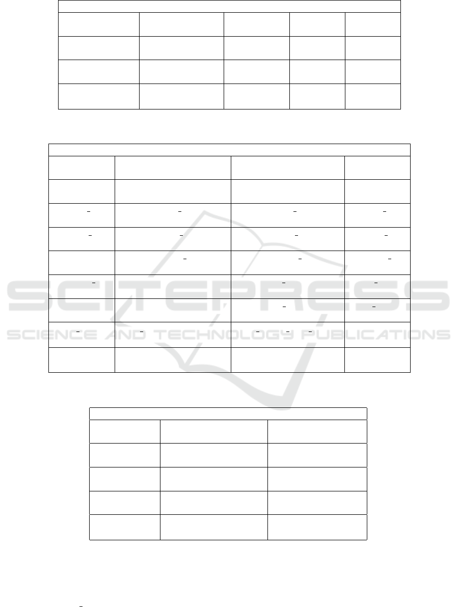
Table 1: Comparison of performance of the randomized neural networks descriptors (

Ω(39) and

Ω(39,49,59)) and its fusion

with other methods (FUSRNN) with other approaches. The compared results were obtained from (Wang et al., 2017).

Approaches and accuracies (%)

Histogram-lower Histogram-higher LBP GLCM Gabor

80.8 72.4 76.2 71.9 63.1

Perception Best2 Best3 Best4 Best5

62.9 85.8 86.0 86.5 87.4

All-6 CNN CNN-H CNN-E BCNN

87.4 90.2 ± 3.1 89.2 ± 1.1 86.1 ± 1.4 92.6 ± 1.2

Ω(39)

Ω(39,49,59) FUSRNN - -

91.34 ± 0.81 92.46 ± 0.44 94.36 ± 0.30 - -

Table 2: Comparison of performance of the randomized neural networks descriptors (

Ω(39) and

Ω(39,49,59)) and its fusion

with other methods (FUSRNN) with other approaches. The compared results were obtained from (Nanni et al., 2019).

Approaches and accuracies (%)

LTP MLPQ CLBP RICLBP

87.6 92.48 90.38 87.88

GOLD HOG AHP FBSIF

84.46 65.60 92.28 92.30

FUS 1 FUS 2 FUS 3 FUS 4

92.24 93.26 93.54 93.74

CLM 1 CLM 2 CLM 3 CLM 4

87.70 86.52 78.02 86.32

CLM CLoVo 1 CLoVo 2 CLoVo 3

85.08 87.26 62.72 86.80

CLoVo 4 CLoVo FUS CLM3 FUS CLM

89.26 89.08 84.82 88.50

DeepOutput DeepScores FUS ND(2) FUS ND(3)

91.90 94.44 92.72 93.02

FUS D(0.5) FUS ND(3)+DeepOutput FUS ND(3) FUS D(0.5)

Ω(39)

94.44 93.24 93.98 91.34 ± 0.81

Ω(39,49,59) FUSRNN - -

92.46 ± 0.44 94.36 ± 0.30 - -

Table 3: Comparison of performance of the randomized neural networks descriptors (

Ω(39) and

Ω(39,49,59)) and its fusion

with other methods (FUSRNN) with other approaches. The compared results were obtained from (Paladini et al., 2021).

Approaches and accuracies (%)

LPQ, SVM BSIF, SVM LPQ+BSIF, SVM

68.12 68.10 74.10

LPQ, NN BSIF, NN LPQ+BSIF, NN

69.02 71.04 74.22

ResNet-101 ResNeXt-50 Inception-v3

95.92 95.74 93.98

DenseNet-161 Mean-Ensemble-CNNs NN-Ensemble-CNNs

95.60 96.16 96.14

Ω(39)

Ω(39,49,59) FUSRNN

91.34 ± 0.81 92.46 ± 0.44 94.36 ± 0.30

son with other approaches, surpasses the performance

of several compared methods in Table 2. The re-

sult of

Ω(39,49,59), in turn, is only surpassed by

more sophisticated approaches based on ensembles

(for instance, FUS 2) or Convolutional Neural Net-

works (for instance, DeepScores). On the other hand,

our proposed signature FUSRNN provided a result

(94.36% ± 0.30%) virtually equivalent to the best per-

formance in Table 2 (DeepScores, with 94.44%).

In Table 3, we performed a comparison with the

Colorectal Image Classiﬁcation Using Randomized Neural Network Descriptors

803

results showed in (Paladini et al., 2021). This table

shows that the three signatures

Ω(39),

Ω(39,49,59)

and FUSRNN largely outperformed all the hand-

crafted methods. On the other hand, almost all

CNN-based approaches surpassed FUSRNN (excep-

tion for Inception-v3), with NN-Ensemble-CNNs pre-

senting an advantage of 1.78%. To explain this

difference in performance, it is important to stress

that the authors in (Paladini et al., 2021) afﬁrm

that ResNet-101, ResNeXt-50, Inception-v3, and

DenseNet-161 are “four of the most powerful CNN

architectures”(Paladini et al., 2021) and that they

used pre-trained models from the ImageNet Chal-

lenge Database. Moreover, the best CNN-based ap-

proach (NN-Ensemble-CNNs) is an ensemble com-

bining the four mentioned CNN architectures.

Finally, the signature

Ω(39,49,59) provides an

accuracy equivalent to ARA-CNN (Raczkowski et al.,

2019) (92.24 ± 0.82%), and the signature FUSRNN

overcomes it. Thus, based on our results, it is pos-

sible to afﬁrm that randomized neural network de-

scriptors (

Ω(39) and

Ω(39,49,59)) have high perfor-

mance, surpassing several texture analysis methods.

Also, when associated with other descriptors (FUS-

RNN), it provided accuracies slightly inferior to the

best CNN architectures. Such performance suggests

that novel improvements in the RNN signature as well

as its association with other descriptors equally dis-

criminative may result in even higher accuracies when

applied to colorectal images.

6 CONCLUSION

This paper presented an application of a highly

discriminative texture descriptor based on weights

of randomized neural network on a very important

multi-class problem, which consists of discriminat-

ing colorectal images into eight classes, according to

the image database provided by (Kather et al., 2016).

The results of the randomized neural network signa-

ture were promising, surpassing several texture analy-

sis methods. When the neural neural descriptors were

associated with other texture analysis methods, this

fusion signature was capable of providing accuracies

similar or slightly inferior to that of several powerful

convolutional neural networks, which are known for

having a high number of parameters to tune. Thus,

ground on our results, we believe that our proposed

applied approach has potential to provide even better

results and adds a valuable tool to the computer vision

research in colorectal images.

ACKNOWLEDGEMENTS

This study was ﬁnanced in part by the Coordenac¸

de Aperfeic¸oamento de Pessoal de N

ıvel Superior

– Brasil (CAPES) – Finance Code 001. Andr

e R.

Backes gratefully acknowledges the ﬁnancial sup-

port of CNPq (Grant #307100/2021-9). Jarbas

Joaci de Mesquita S

a Junior thanks Coordenac¸

de Aperfeic¸oamento de Pessoal de N

ıvel Superior

(CAPES, Brazil) for the ﬁnancial support of this

work.

REFERENCES

Backes, A. R., Casanova, D., and Bruno, O. M. (2013). Tex-

ture analysis and classiﬁcation: A complex network-

based approach. Information Sciences, 219:168 – 180.

Boser, B. E., Guyon, I. M., and Vapnik, V. N. (1992). A

training algorithm for optimal margin classiﬁers. In

Proceedings of the Fifth Annual Workshop on Compu-

tational Learning Theory, pages 144–152. ACM.

Calvetti, D., Morigi, S., Reichel, L., and Sgallari, F. (2000).

Tikhonov regularization and the l-curve for large dis-

crete ill-posed problems. Journal of Computational

and Applied Mathematics, 123(1):423–446.

Chang, C.-C. and Lin, C.-J. (2011). LIBSVM: A library

for support vector machines. ACM Transactions on

Intelligent Systems and Technology, 2:27:1–27:27.

Cortes, C. and Vapnik, V. (1995). Support-vector networks.

Machine Learning, 20(3):273–297.

Cover, T. M. (1965). Geometrical and statistical properties

of systems of linear inequalities with applications in

pattern recognition. IEEE Transactions on Electronic

Computers, EC-14(3):326–334.

Daugman, J. and Downing, C. (1995). Gabor wavelets for

statistical pattern recognition. In Arbib, M. A., edi-

tor, The Handbook of Brain Theory and Neural Net-

works, pages 414–419. MIT Press, Cambridge, Mas-

sachusetts.

dos Santos, L. F. S., Neves, L. A., Rozendo, G. B., Ribeiro,

M. G., do Nascimento, M. Z., and Tosta, T. A. A.

(2018). Multidimensional and fuzzy sample entropy

(SampEnMF) for quantifying H&E histological im-

ages of colorectal cancer. Computers in Biology and

Medicine, 103:148 – 160.

Haﬁane, A., Palaniappan, K., and Seetharaman, G. (2015).

Joint adaptive median binary patterns for texture clas-

siﬁcation. Pattern Recognition, 48(8):2609–2620.

Huang, G.-B., Zhu, Q.-Y., and Siew, C.-K. (2006). Extreme

learning machine: theory and applications. Neuro-

computing, 70(1):489–501.

Kather, J. N., Weis, C.-A., Bianconi, F., Melchers, S. M.,

Schad, L. R., Gaiser, T., Marx, A., and Zollner,

F. G. (2016). Multi-class texture analysis in colorec-

tal cancer histology. Scientiﬁc Reports, 6(27988).

doi:10.1038/srep27988.

VISAPP 2024 - 19th International Conference on Computer Vision Theory and Applications

804

Manjunath, B. S. and Ma, W.-Y. (1996). Texture features

for browsing and retrieval of image data. IEEE Trans.

Pattern Anal. Mach. Intell, 18(8):837–842.

Moore, E. H. (1920). On the reciprocal of the general alge-

braic matrix. Bulletin of the American Mathematical

Society, 26:394–395.

Nanni, L., Brahnam, S., Ghidoni, S., and Lumini, A. (2019).

Bioimage classiﬁcation with handcrafted and learned

features. IEEE/ACM Transactions on Computational

Biology and Bioinformatics, 16(3):874–885.

Ojala, T., Pietik

ainen, M., and M

aenp

a, T. (2002). Mul-

tiresolution gray-scale and rotation invariant texture

classiﬁcation with local binary patterns. IEEE Trans.

Pattern Anal. Mach. Intell, 24(7):971–987.

Paladini, E., Vantaggiato, E., Bougourzi, F., Distante,

C., Hadid, A., and Taleb-Ahmed, A. (2021). Two

ensemble-CNN approaches for colorectal cancer tis-

sue type classiﬁcation. Journal of Imaging, 7(3).

Pao, Y.-H., Park, G.-H., and Sobajic, D. J. (1994). Learning

and generalization characteristics of the random vec-

tor functional-link net. Neurocomputing, 6(2):163–

180.

Pao, Y.-H. and Takefuji, Y. (1992). Functional-link net com-

puting: theory, system architecture, and functionali-

ties. Computer, 25(5):76–79.

Penrose, R. (1955). A generalized inverse for matrices.

Mathematical Proceedings of the Cambridge Philo-

sophical Society, 51(3):406–413.

Peyret, R., Bouridane, A., Kheliﬁ, F., Tahir, M. A., and

Al-Maadeed, S. (2018). Automatic classiﬁcation of

colorectal and prostatic histologic tumor images us-

ing multiscale multispectral local binary pattern tex-

ture features and stacked generalization. Neurocom-

puting, 275:83 – 93.

Raczkowski, L., Mozejko, M., Zambonelli, J., and

Szczurek, E. (2019). ARA: accurate, reliable and

active histopathological image classiﬁcation frame-

work with Bayesian deep learning. Scientiﬁc Reports,

9(14347).

Ribeiro, M. G., Neves, L. A., Nascimento, M. Z., Roberto,

G. F., Martins, A. S., and Tosta, T. A. A. (2019). Clas-

siﬁcation of colorectal cancer based on the association

of multidimensional and multiresolution features. Ex-

pert Systems with Applications, 120:262 – 278.

a Junior, J. J. M. and Backes, A. R. An improved ran-

domized neural network signature for texture classiﬁ-

cation. SSRN.

a Junior, J. J. M. and Backes, A. R. (2016). ELM based

signature for texture classiﬁcation. Pattern Recogni-

tion, 51:395–401.

Schmidt, W. F., Kraaijveld, M. A., and Duin, R. P. W.

(1992). Feedforward neural networks with random

weights. In Proceedings., 11th IAPR International

Conference on Pattern Recognition. Vol.II. Confer-

ence B: Pattern Recognition Methodology and Sys-

tems, pages 1–4.

Siegel, R. L., Miller, K. D., Wagle, N. S., and Jemal, A.

(2023). Cancer statistics, 2023. CA: A Cancer Journal

for Clinicians, 73(1):17–48.

Tikhonov, A. N. (1963). On the solution of ill-posed prob-

lems and the method of regularization. Dokl. Akad.

Nauk SSSR, 151(3):501–504.

Wang, C., Shi, J., Zhang, Q., and Ying, S. (2017).

Histopathological image classiﬁcation with bilinear

convolutional neural networks. In 2017 39th Annual

International Conference of the IEEE Engineering in

Medicine and Biology Society (EMBC), pages 4050–

4053.

Weszka, J. S., Dyer, C. R., and Rosenfeld, A. (1976). A

comparative study of texture measures for terrain clas-

siﬁcation. IEEE Trans. Syst., Man, Cyb., 6(4):269–

285.

Yoon, H., Lee, J., Oh, J. E., Kim, H. R., Lee, S., Chang,

H. J., and Sohn, D. K. (2019). Tumor identiﬁcation in

colorectal histology images using a convolutional neu-

ral network. Journal of Digital Imaging, 32(1):131–

140.

Colorectal Image Classiﬁcation Using Randomized Neural Network Descriptors

805