PatchSVD: A Non-Uniform SVD-Based Image Compression Algorithm

Zahra Golpayegani and Nizar Bouguila

Gina Cody School of Engineering, Concordia University, Montreal, Canada

Keywords:

Lossy Image Compression, Singular Value Decomposition, PatchSVD, Joint Photographic Experts Group.

Abstract:

Storing data is particularly a challenge when dealing with image data which often involves large ﬁle sizes

due to the high resolution and complexity of images. Efﬁcient image compression algorithms are crucial to

better manage data storage costs. In this paper, we propose a novel region-based lossy image compression

technique, called PatchSVD, based on the Singular Value Decomposition (SVD) algorithm. We show through

experiments that PatchSVD outperforms SVD-based image compression with respect to three popular im-

age compression metrics. Moreover, we compare PatchSVD compression artifacts with those of Joint Photo-

graphic Experts Group (JPEG) and SVD-based image compression and illustrate some cases where PatchSVD

compression artifacts are preferable compared to JPEG and SVD artifacts.

1 INTRODUCTION

Enormous amounts of data are generated every day

by various sources, including social media, sensors on

wearable devices, and smart gadgets. In many cases,

the data needs to be stored on a small device to serve

a speciﬁc purpose. For instance, a real-time defect

detector stores images of its camera feed and sends

them to a lightweight model to catch possible ﬂaws

in a production line (Pham et al., 2023). Such small

devices are limited in storage capacities; therefore, it

is essential to design efﬁcient data storage algorithms

capable of storing the data without signiﬁcant loss in

quality.

Images are one of the most commonly used data

formats, and storing an image ﬁle on a digital device

can require anywhere from kilobytes to megabytes of

storage space, depending on the complexity of the im-

age and the storage technique. Image compression

algorithms can be categorized into lossless and lossy

compression methods. In lossless methods, such as

Portable Network Graphics (PNG) image compres-

sion, the original input can be reconstructed after

compressing because compression was achieved by

removing statistical redundancies. However, only low

compression ratios are achievable through lossless

image compression, and image compression is not al-

ways guaranteed. On the other hand, lossy compres-

sion techniques, such as Joint Photographic Experts

Group (JPEG) compression (Wallace, 1991), achieve

higher compression ratios by allowing more informa-

Figure 1: JPEG produces more compression artifacts in im-

ages containing text compared to the proposed method. The

sample is taken from the IAM Handwriting Database and

the image has been zoomed in 30 times the original size to

better visualize the compression artifacts.

tion loss, but the reconstructed image sometimes con-

tains visible compression artifacts. Speciﬁcally, JPEG

image compression is based on the assumption that

within an 8×8 pixel block, there are no sharp changes

in intensity. However, in some use cases, such as

compressing images of text or electronic circuit di-

agrams, this assumption does not hold, and JPEG cre-

ates visible compression artifacts around the drawn

lines. Figure 1 compares the JPEG compression ar-

tifacts with those of the proposed method presented

886

Golpayegani, Z. and Bouguila, N.

PatchSVD: A Non-Uniform SVD-Based Image Compression Algorithm.

DOI: 10.5220/0012488500003654

Paper published under CC license (CC BY-NC-ND 4.0)

In Proceedings of the 13th International Conference on Pattern Recognition Applications and Methods (ICPRAM 2024), pages 886-893

ISBN: 978-989-758-684-2; ISSN: 2184-4313

in this paper, using an example image containing text

sourced from the IAM Handwriting Database (Marti

and Bunke, 2002).

To improve the compression results, some tradi-

tional methods compress regions of interest (ROIs)

with a higher bit-rate than the rest of the regions

(Christopoulos et al., 2000), however, the ROIs are

not detected automatically and should be speciﬁed

by the user. Deep learning-based approaches have

also been applied to image compression (Cheng et al.,

2018; Toderici et al., 2017; Agustsson et al., 2017; Li

et al., 2018; Cheng et al., 2019; Prakash et al., 2017).

Nevertheless, training deep learning models require

high computational power and during inference, the

model has to exist on the device that runs the com-

pression code, which calls for additional storage com-

pared to traditional methods.

In this paper, we propose a new image com-

pression algorithm based on Singular Value Decom-

position (SVD), called PatchSVD

. First, we ex-

plain how PatchSVD works, what is the compres-

sion ratio we can achieve using PatchSVD, and what

are the required conditions to compress an image

using PatchSVD. Then, through extensive experi-

ments, we demonstrate that PatchSVD outperforms

SVD in terms of Structural Similarity Index Mea-

sure (SSIM), Peak Signal-to-Noise Ratio (PSNR),

and Mean Squared Error (MSE) metrics. Moreover,

through examples, we show that PatchSVD is more

robust against sharp pixel intensity changes, there-

fore, it is preferable over JPEG in some use cases,

including compressing images of text, where high

changes in pixel intensity exist.

2 PRELIMINARIES

In this section, we brieﬂy overview SVD and its basic

properties. Singular Value Decomposition or SVD is

an algorithm that factorizes a given matrix A ∈ R

m×n

into three components A = USV

, where U

m×m

and

n×n

are orthogonal matrices and S

m×n

is a diagonal

matrix containing singular values in descending or-

der. The singular values are non-negative real num-

bers that represent the magnitude of the singular vec-

tors; i.e., larger singular values indicate directions in

the data space where there is more variability. There-

fore, by keeping the larger singular values and their

corresponding vectors, the original matrix can be ap-

proximated with minimum information loss.

The maximum number of linearly independent

rows or columns of a matrix is called the rank (r) of

PatchSVD source code is available at https://github.c

om/zahragolpa/PatchSVD

that matrix. When a matrix A is decomposed using

SVD, the number of non-zero elements on the diag-

onal of S is equal to r. By retaining only the ﬁrst r

elements from U, S, and V

we get an r-rank approx-

imation A

= U

for the matrix A.

If we use k-rank SVD to compress an image rep-

resented by matrix A

m×n

, the number of elements we

need to store to represent the compressed image is cal-

culated by summing up the number of elements from

each SVD component. Therefore, storing the k-rank

version of A

m×n

with m × n elements only requires

SV D

= k (m + n + 1) values. Note that the k-rank

approximation of matrix A keeps most of the use-

ful information about the image while reducing the

storage requirements for the input, especially if the

rows and columns in the image are highly correlated

(r ≪ min(m, n)). However, when higher compression

ratios are required, it is beneﬁcial to sacriﬁce more

information to save more storage, which is achievable

by choosing k

SV D

< k.

3 RELATED WORKS

SVD has been used before in literature for image

compression (Andrews and Patterson, 1976; Akri-

tas and Malaschonok, 2004; Kahu and Rahate, 2013;

Prasantha et al., 2007; Tian et al., 2005; Cao, 2006).

In (Ranade et al., 2007), a variation on image com-

pression using SVD has been proposed that applies a

data-independent permutation on the input image be-

fore performing SVD-based image compression as a

preprocessing step. In (Sadek, 2012), a forensic tool

is developed using SVD that embeds a watermark

into the image noise subspace. Another application

of SVD applied to image data is image recovery dis-

cussed in (Chen, 2018) where authors used SVD for

matrix completion.

Few studies have investigated region-based or

patch-based image compression using techniques

similar to SVD. In (Lim et al., 2014), a GUI system is

designed that takes Regions of Interest (ROI) in med-

ical images to ensure near-zero information loss in

those regions compared to the rest of the image when

compressed. However, users need to select the ROIs

manually, and Principle Component Analysis (PCA)

is used instead of SVD. (Lim and Abd Manap, 2022)

used a patch-based PCA algorithm that eliminates the

need to manually select the ROIs in brain MRI scans

using the brain symmetrical property. However, their

approach has very limited use cases because of the

assumed symmetrical property in the images.

Joint Photographic Experts Group (JPEG) com-

pression (Wallace, 1991) is one of the most com-

PatchSVD: A Non-Uniform SVD-Based Image Compression Algorithm

887

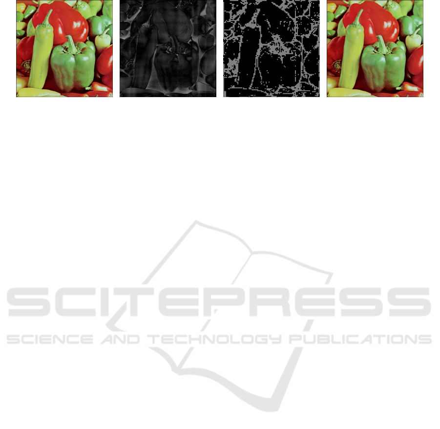
(a) Original image (b) Difference image (∆) (c) Complex (in gray) and

simple (in black) patches

(d) PatchSVD output

Figure 2: PatchSVD algorithm ﬁrst applies low-rank SVD to the original image and subtracts the low-rank approximation

from the original image (Figure 2(a)) to obtain ∆ (Figure 2(b)). Then, by applying a score function, PatchSVD calculates the

patches that contain more information according to ∆ (2(c)) to create the ﬁnal compressed image (see Figure 2(d)).

monly used image compression methods, applicable

to both grayscale and color continuous-tone images.

JPEG works by transforming an image from the spa-

tial domain to the frequency domain using Discrete

Cosine Transforms (DCTs) (Ahmed et al., 1974).

Each image is divided into 8 × 8 pixels blocks, trans-

formed using DCT, and then quantized according to

a quantization table, followed by further compression

using an entropy encoding algorithm, such as Huff-

man coding (Huffman, 1952). While JPEG is used

in many use cases, it fails to perform well in exam-

ples where sudden changes in intensity exist within

the blocks.

We aim to extend the previous works by automati-

cally selecting the complex patches and utilizing SVD

with respect to the image context to compress images

with minimum information loss and achieve signif-

icant reductions in storage without any training re-

quired using simple mathematical operations.

4 METHOD

4.1 PatchSVD Algorithm

To compress A

m×n

using PatchSVD, we ﬁrst compute

the SVD of the image and take the ﬁrst k

SV D

singu-

lar values to reconstruct the k

SV D

-rank approximation.

Then, we subtract the k

SV D

-rank approximation from

the original image to get matrix ∆ (see Figure 2(b)).

In our experiments, we selected the initial k

SV D

= 1.

Based on the properties of SVD, the k

SV D

-rank ap-

proximation captures most of the image information;

therefore, high values in ∆ (white pixels) indicate pix-

els that were not captured by the ﬁrst singular values,

and low values in ∆ (black pixels) would give us those

locations were almost all the information in the origi-

nal image was captured by the k

SV D

-rank approxima-

tion. Therefore, to distinguish the complex patches

that SVD missed from the simpler ones, we investi-

gate the values in ∆ and determine if a patch is com-

plex or simple (see Figure 2(c)). In other words, the

∆ matrix helps us ﬁnd the areas that would introduce

large compression errors if we used the standard SVD

for image compression. We utilize ∆ as a heuristic

function to minimize the compression error by apply-

ing non-uniform compression.

More speciﬁcally, we split the image correspond-

ing to the ∆ matrix into patches of size P

× P

. If the

image is not divisible by the patch dimensions, we

add temporary margins to the sides with pixel values

equal to the average pixel value in the image. Then,

we loop over the patches and assign a score to each

patch according to a score function. Next, we sort

the patches based on the score and select the top n

complex patches. The number of complex patches is

determined based on the desired compression ratio,

following Equation 2.

After we ﬁnd the complex patches, we run SVD

for each patch and take the k-rank approximation with

two different constants; k

for complex patches and

for simple patches where k

≤ k

. When we en-

counter the patches that contain the extra margin, we

remove the margin before performing k-rank approx-

imation using SVD. Finally, we put the compressed

patches together to form the compressed image (see

Figure 2(d)). PatchSVD algorithm is described in

detail in Algorithm 1. We argue that PatchSVD is

a more ﬂexible image compression algorithm com-

pared to SVD and JPEG because it allows you to as-

sign non-uniform importance to each patch in the im-

age according to a customizable function. While our

method relies on the 1-rank SVD to calculate the ∆

matrix and employs the standard deviation score func-

tion to sort patches, it is noteworthy that various tech-

niques, such as graph-based approaches, gradient-

based methods, edge detection, and expert knowl-

edge, can also be employed to detect and sort com-

ICPRAM 2024 - 13th International Conference on Pattern Recognition Applications and Methods

888

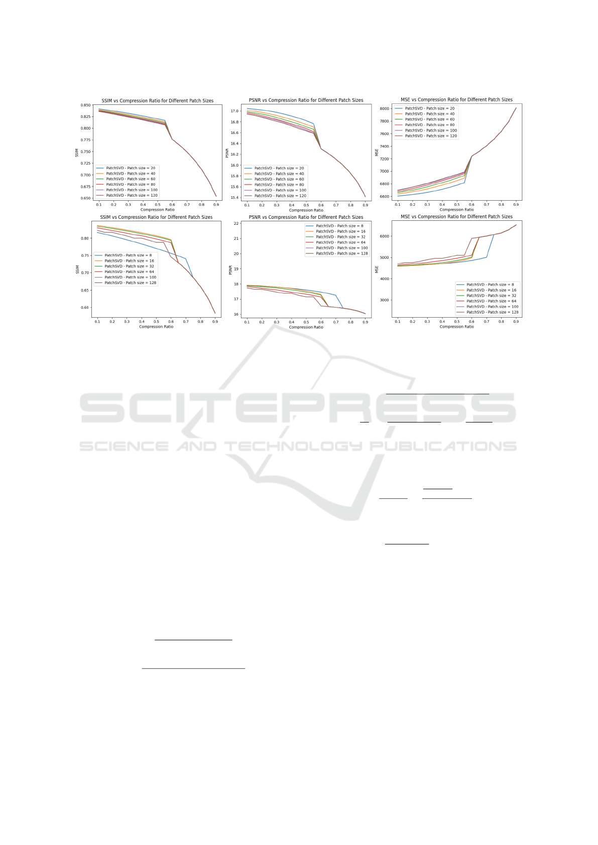
Figure 3: This ﬁgure shows the effect of patch size on the performance of the PatchSVD algorithm across CLIC (ﬁrst row)

and Kodak (second row) datasets.

plex patches. The choice may depend on the speciﬁc

requirements of the application.

4.2 Compression Ratio (CR)

Suppose we want to compress an input image of size

m × n using PatchSVD and we choose the patch size

to be P

× P

. The amount of compression we get

depends on the values we choose for k

and k

, i.e.,

lower-rank approximations result in higher amounts

of image compression. More speciﬁcally, the number

of digits we need to save, S

PatchSVD

, to represent an

image using PatchSVD is S

PatchSVD

= n

+ P

1)+n

+1), where n

and n

are the number

of complex and simple patches, respectively. Taking

= k

SVD

would result in the storage required

by the SVD algorithm (S

SVD

) which is equivalent to

the storage needed by the PatchSVD algorithm when

= n, P

= m, n

= 1, and n

= 0 which is equal to

SVD

= k

SVD

(m + n + 1).

Therefore, the Compression Ratio (CR) can be

calculated using the following formula:

CR =

Original

− S

PatchSVD

Original

= 1 −

+ P

+ 1)(n

+ n

)

+ n

)

(1)

where S

Original

is the storage needed for the original

image. From 1, we can calculate the number of com-

plex patches n

when the required compression ratio

is known:

CR = 1 −

+ P

+ 1)(n

+ n

)

+ n

)

=⇒

= (

(1 −CR)

+ P

+ 1

− k

)

− k

(2)

where t is the total number of patches in the image.

We need to ensure CR ≥ 0 to have a compressed im-

age; therefore, the following should hold:

0 ≤

+ n

≤

− k

(3)

which requires two conditions to be true:

+ P

+ 1

≥ k

(4)

and

≥ k

(5)

Moreover, we can observe from the condition in

3 that there is a trade-off between the proportion of

the complex patches and the values we choose for k

and k

. For instance, if we want to keep a higher pro-

portion of complex patches, the difference between k

and k

should be higher and k

should be much smaller

than k

. Note that since k

≥ k

≥ 0, the proportion of

complex patches cannot be higher than a threshold.

On the other hand, if the proportion is too small, the

number of complex patches may end up being less

than 1, in which case PatchSVD will fall back to the

standard SVD-based image compression algorithm.

PatchSVD: A Non-Uniform SVD-Based Image Compression Algorithm

889

Input: A

m×n

, k

, P

, CR

Output: cmpr image

← (

(1−CR)

− k

)

−k

;

∆ ← A − k rank SVD(A, 1);

∆

patches

← patch and add margin(∆, P

, P

);

× num patches < 1 then

k SVD ← int((1 − CR) ×

m×n

m+n+1

);

return k rank SVD(A, k SVD);

end

for patch in ∆

patches

∆

scores

[patch] ← score(patch);

end

∆

scores

← sort(∆

scores

);

for patch in ∆

patches

U, S,V

← SVD(patch);

if index(patch) ≤ n

then

k ← k

;

end

else

k ← k

;

end

cmpr patch ← k rank SVD(patch, k);

cmpr patches.append(cmpr patch);

end

cmpr image ← arrange(cmpr patches);

return cmpr image;

Algorithm 1: PatchSVD Image Compression.

4.3 Patch Size Lower Bound

Not every arbitrary patch size works with the

PatchSVD algorithm. While the image size is a triv-

ial upper bound for P, it should be noted that greater

patch sizes will result in less accurate scoring. More

speciﬁcally, if the patch size is too large, the score

function will lose its sensitivity to complex versus

simple patches because of its less local domain. To

ﬁnd a lower bound for patch size, we simplify Equa-

tion 4 by assuming that we are using a square patch

with P

= P

= P. Then, we will have

2P+1

≥ k

By simplifying this inequality further, we get a

lower bound on the patch size which is P ≥ k

+ k

≥ 0.

5 EXPERIMENTS

With PatchSVD, we compress images from two

datasets using different patch sizes to evaluate the ef-

fect of patch size on the performance of the algorithm.

Then, we pick the best patch size for each dataset and

compare PatchSVD with SVD and JPEG according to

three metrics and by visually comparing the compres-

sion artifacts. We also brieﬂy discuss some choices

for PatchSVD score functions and how they compare

with each other.

5.1 Datasets and Metrics

We evaluated our method on Kodak (Kodak, 1999)

and CLIC (Toderici et al., 2020) datasets because

they contain original PNG format images that were

never converted to JPEG. Kodak is a classic dataset

that is frequently used for evaluating image compres-

sion algorithms. It contains 24 full-color (24 bits per

pixel) images that are either 768x512 or 512x768 pix-

els large. The images in this dataset capture a variety

of lighting conditions and contain different subjects.

The CLIC dataset was introduced in the lossy image

compression track for the Challenge on Learned Im-

age Compression in 2020 and includes both RGB and

grayscale images. For all the experiments, we utilized

the test split, which comprises 428 samples.

We use traditional image compression metrics, in-

cluding Mean Squared Error (MSE), Peak Signal-

to-noise Ratio (PSNR), and Structural Similarity In-

dex Measure (SSIM) (Wang et al., 2004) to evaluate

the image compression performance of each method.

Lower MSE means better performance, indicating re-

duced pixel deviations. Higher PSNR and SSIM val-

ues signal superior image quality with less distortion

and increased similarity between original and pro-

cessed images.

6 RESULTS AND DISCUSSION

6.1 PatchSVD Performance Based on

Patch Size

Figure 3 depicts the impact of patch size on the perfor-

mance of the PatchSVD algorithm across the Kodak

and CLIC datasets, as measured by SSIM, PSNR, and

MSE metrics. The ﬁndings indicate that opting for ex-

cessively large patch sizes is not advisable, and the ef-

fectiveness of compression may be compromised with

patch sizes that are too small, contingent on the char-

acteristics of the dataset. Note that the algorithm falls

back to SVD for patch sizes that are too large which

is why the plots overlap for some compression ratios.

6.2 Image Compression Performance

Comparison

To better demonstrate the performance of PatchSVD,

we compared the performance of PatchSVD with a

ICPRAM 2024 - 13th International Conference on Pattern Recognition Applications and Methods

890

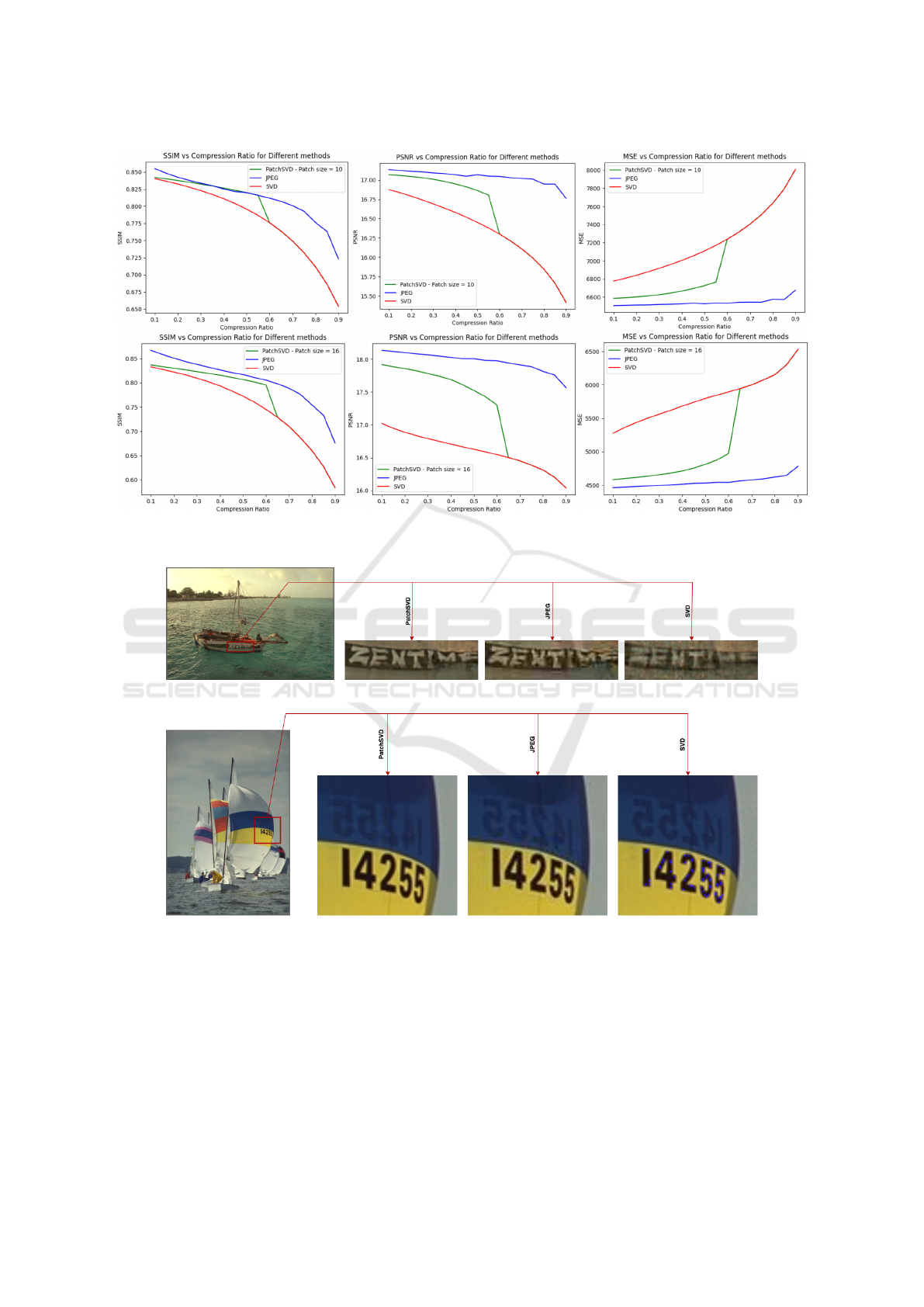
Figure 4: This ﬁgure compares SSIM, PSNR, and MSE metrics for PatchSVD, JPEG, and SVD image compression algorithms

on the CLIC dataset with a patch size of 10 (top row) and the Kodak dataset with a patch size of 16 (bottom row).

(a) Image compression at CR = 85% applied to ”kodim06.png” from the Kodak dataset.

(b) Image compression at CR = 20% applied to ”kodim09.png” from the Kodak dataset.

Figure 5: PatchSVD, JPEG, and SVD compression algorithms applied to two image samples from the Kodim dataset show

the compression artifacts produced by each algorithm. As you can see, PatchSVD produces more sharp edges which results

in perfectly legible text even after the image has been greatly compressed.

ﬁxed patch size against JPEG and SVD on CLIC and

Kodak datasets. According to the experiment results

in Section 6.1, patch sizes 10 and 16 were selected for

CLIC and Kodak, respectively. Figure 4 illustrates

the performance comparison with respect to SSIM,

PSNR, and MSE. PatchSVD outperforms SVD in all

three metrics on both datasets, although JPEG still

performs better than PatchSVD. This is expected be-

cause neither of the three metrics are context-aware.

Nevertheless, PatchSVD may still be preferred over

JPEG in some use cases as explained in Section 6.3.

PatchSVD: A Non-Uniform SVD-Based Image Compression Algorithm

891

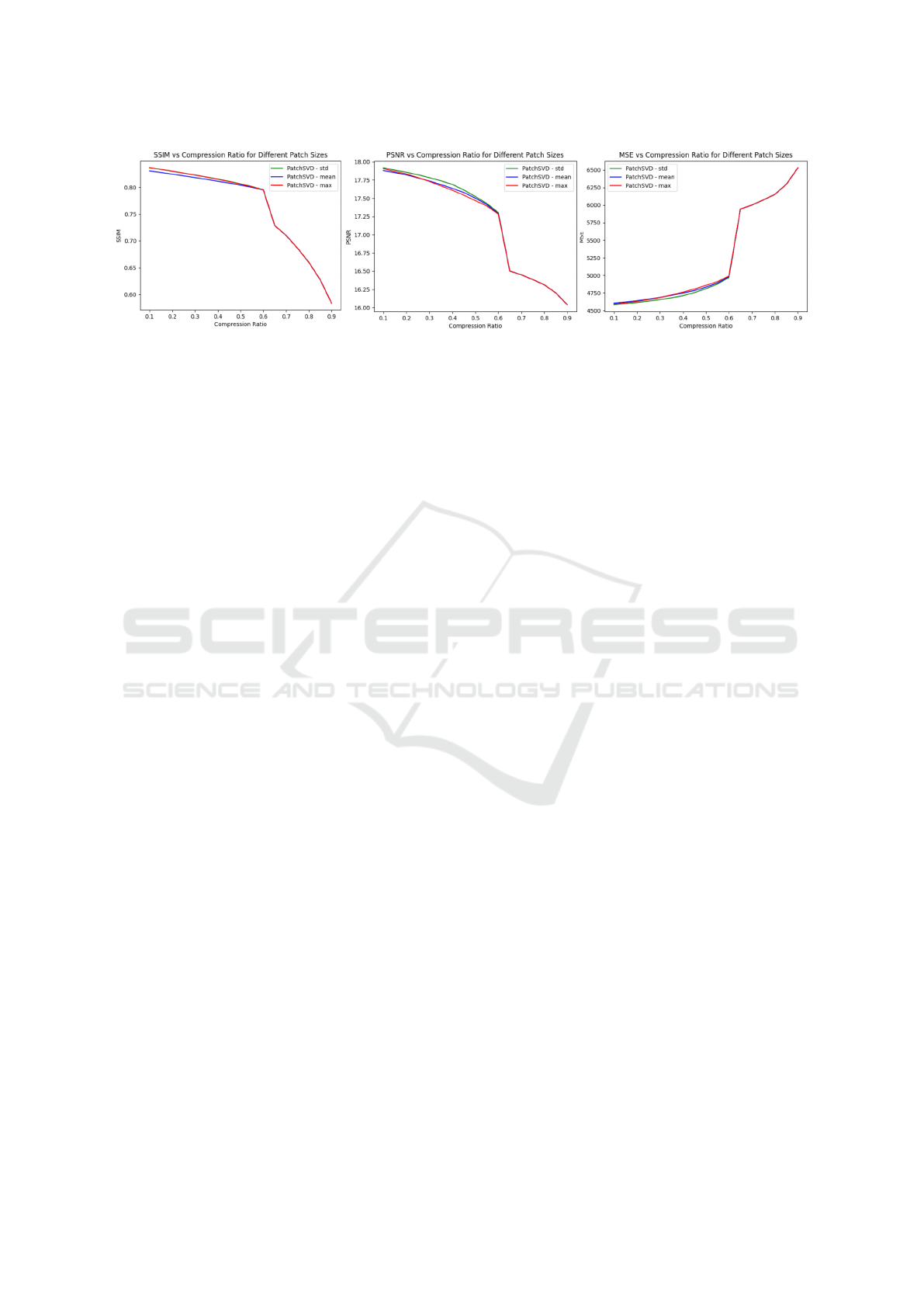
Figure 6: This ﬁgure illustrates PatchSVD algorithm performance on the Kodak dataset with the patch size of 16 using

different score functions, namely, standard deviation (std), mean, and maximum (max). To compare, SSIM, PSNR, and MSE

metrics are used. It is demonstrated that standard deviation has a slightly better performance compared to others.

6.3 Compression Artifacts

While the compression artifacts of PatchSVD and

SVD are usually in the form of colored pixels (some-

times called ”stuck pixels”, see SVD output in Fig-

ure 5(b)), for JPEG, these artifacts take the forms of a

general loss of sharpness and visible halos around the

edges in the image. In higher compression ratios, the

edges of blocks that PatchSVD and JPEG use become

visible, too. However, for use cases where sharpness

should be maintained locally, PatchSVD is preferable.

For example, in Figure 5, for both samples, the text

written on the boat is more legible when the image is

compressed with PatchSVD.

6.4 Choice of Score Function

We compared various score functions, including tak-

ing the maximum value, averaging, and calculating

the standard deviation of the pixel values present in

the input patch, as shown in Figure 6. The perfor-

mance of all the score functions is almost similar,

but standard deviation yields better results in terms

of SSIM, PSNR, and MSE. The intuition behind this

is that standard deviation introduces sensitivity to de-

viations from the mean which is usually where more

complex patterns are present.

7 CONCLUSION

In this work, we introduced PatchSVD as a non-

uniform image compression algorithm based on SVD.

Through experiments, we demonstrated that the patch

size in the PatchSVD algorithm affects the compres-

sion performance. Also, we compared the perfor-

mance of PatchSVD with JPEG and SVD with re-

spect to SSIM, PSNR, and MSE. We compared the

compression artifacts that each algorithm introduced

to images and illustrated examples of the cases where

PatchSVD was preferable over JPEG and SVD be-

cause it produced less destructive artifacts in regions

that contained information that would have been lost

if we applied standard SVD-based image compres-

sion. Studying the impact of PatchSVD as an im-

age compression algorithm on the downstream tasks

is an interesting future work. Moreover, applying

PatchSVD to medical images is a prospective exten-

sion because, in medical images, higher resolution

is required in the pixels containing diagnostic infor-

mation compared to the rest of the image and non-

uniform local compression could be beneﬁcial. Ex-

pert knowledge can lead us to more customized score

functions which makes this application even more in-

teresting.

REFERENCES

Agustsson, E., Mentzer, F., Tschannen, M., Cavigelli, L.,

Timofte, R., Benini, L., and Gool, L. V. (2017). Soft-

to-hard vector quantization for end-to-end learning

compressible representations. Advances in neural in-

formation processing systems, 30.

Ahmed, N., Natarajan, T., and Rao, K. R. (1974). Discrete

cosine transform. IEEE transactions on Computers,

100(1):90–93.

Akritas, A. G. and Malaschonok, G. I. (2004). Applications

of singular-value decomposition (svd). Mathematics

and computers in simulation, 67(1-2):15–31.

Andrews, H. and Patterson, C. (1976). Singular value de-

composition (svd) image coding. IEEE transactions

on Communications, 24(4):425–432.

Cao, L. (2006). Singular value decomposition applied

to digital image processing. Division of Computing

Studies, Arizona State University Polytechnic Cam-

pus, Mesa, Arizona State University polytechnic Cam-

pus, pages 1–15.

Chen, Z. (2018). Singular value decomposition and its

applications in image processing. In Proceedings of

ICPRAM 2024 - 13th International Conference on Pattern Recognition Applications and Methods

892

the 2018 1st International Conference on Mathemat-

ics and Statistics, pages 16–22.

Cheng, Z., Sun, H., Takeuchi, M., and Katto, J. (2018).

Deep convolutional autoencoder-based lossy image

compression. In 2018 Picture Coding Symposium

(PCS), pages 253–257. IEEE.

Cheng, Z., Sun, H., Takeuchi, M., and Katto, J. (2019).

Deep residual learning for image compression. In

CVPR Workshops, page 0.

Christopoulos, C., Skodras, A., and Ebrahimi, T. (2000).

The jpeg2000 still image coding system: an

overview. IEEE transactions on consumer electron-

ics, 46(4):1103–1127.

Huffman, D. A. (1952). A method for the construction of

minimum-redundancy codes. Proceedings of the IRE,

40(9):1098–1101.

Kahu, S. and Rahate, R. (2013). Image compression

using singular value decomposition. International

Journal of Advancements in Research & Technology,

2(8):244–248.

Kodak (1999). Kodak lossless true color image suite. Last

accessed on 2023-11-14.

Li, M., Zuo, W., Gu, S., Zhao, D., and Zhang, D.

(2018). Learning convolutional networks for content-

weighted image compression. In Proceedings of

the IEEE conference on computer vision and pattern

recognition, pages 3214–3223.

Lim, S. T. and Abd Manap, N. B. (2022). A region-based

compression technique for medical image compres-

sion using principal component analysis (pca). Inter-

national Journal of Advanced Computer Science and

Applications, 13(2).

Lim, S. T., Yap, D. F., and Manap, N. (2014). A gui sys-

tem for region-based image compression using princi-

pal component analysis. In 2014 International Con-

ference on Computational Science and Technology

(ICCST), pages 1–4. IEEE.

Marti, U.-V. and Bunke, H. (2002). The iam-database:

an english sentence database for ofﬂine handwrit-

ing recognition. International Journal on Document

Analysis and Recognition, 5:39–46.

Pham, D.-L., Chang, T.-W., et al. (2023). A yolo-based

real-time packaging defect detection system. Procedia

Computer Science, 217:886–894.

Prakash, A., Moran, N., Garber, S., DiLillo, A., and Storer,

J. (2017). Semantic perceptual image compression us-

ing deep convolution networks. In 2017 Data Com-

pression Conference (DCC), pages 250–259. IEEE.

Prasantha, H., Shashidhara, H., and Murthy, K. B. (2007).

Image compression using svd. In International con-

ference on computational intelligence and multimedia

applications (ICCIMA 2007), volume 3, pages 143–

145. IEEE.

Ranade, A., Mahabalarao, S. S., and Kale, S. (2007). A

variation on svd based image compression. Image and

Vision computing, 25(6):771–777.

Sadek, R. A. (2012). SVD based image processing appli-

cations: State of the art, contributions and research

challenges. CoRR, abs/1211.7102.

Tian, M., Luo, S.-W., and Liao, L.-Z. (2005). An inves-

tigation into using singular value decomposition as a

method of image compression. In 2005 International

Conference on Machine Learning and Cybernetics,

volume 8, pages 5200–5204. IEEE.

Toderici, G., Shi, W., Timofte, R., Theis, L., Balle, J.,

Agustsson, E., Johnston, N., and Mentzer, F. (2020).

Workshop and challenge on learned image compres-

sion (clic2020). Last accessed on 2023-11-14.

Toderici, G., Vincent, D., Johnston, N., Jin Hwang, S.,

Minnen, D., Shor, J., and Covell, M. (2017). Full

resolution image compression with recurrent neural

networks. In Proceedings of the IEEE conference

on Computer Vision and Pattern Recognition, pages

5306–5314.

Wallace, G. K. (1991). The jpeg still picture compression

standard. Communications of the ACM, 34(4):30–44.

Wang, Z., Bovik, A. C., Sheikh, H. R., and Simoncelli, E. P.

(2004). Image quality assessment: from error visi-

bility to structural similarity. IEEE transactions on

image processing, 13(4):600–612.

PatchSVD: A Non-Uniform SVD-Based Image Compression Algorithm

893