iXGB: Improving the Interpretability of XGBoost Using Decision Rules
and Counterfactuals
Mir Riyanul Islam
∗ a
, Mobyen Uddin Ahmed
b
and Shahina Begum
c
Artificial Intelligence and Intelligent Systems Research Group, School of Innovation Design and Engineering,
M
¨
alardalen University, Universitetsplan 1, 722 20 V
¨
aster
˚
as, Sweden
Keywords:
Counterfactuals, Explainability, Explainable Artificial Intelligence, Interpretability, Regression, Rule-Based
Explanation, XGBoost.
Abstract:
Tree-ensemble models, such as Extreme Gradient Boosting (XGBoost), are renowned Machine Learning
models which have higher prediction accuracy compared to traditional tree-based models. This higher
accuracy, however, comes at the cost of reduced interpretability. Also, the decision path or prediction rule
of XGBoost is not explicit like the tree-based models. This paper proposes the iXGB–interpretable XGBoost,
an approach to improve the interpretability of XGBoost. iXGB approximates a set of rules from the internal
structure of XGBoost and the characteristics of the data. In addition, iXGB generates a set of counterfactuals
from the neighbourhood of the test instances to support the understanding of the end-users on their operational
relevance. The performance of iXGB in generating rule sets is evaluated with experiments on real and
benchmark datasets, which demonstrated reasonable interpretability. The evaluation result also supports the
idea that the interpretability of XGBoost can be improved without using surrogate methods.
1 INTRODUCTION
Tree-ensemble is a class of Machine Learning (ML)
models which have gained recent popularity for their
efficacy in handling a diverse array of tabular data
in real-world applications (Sagi and Rokach, 2021).
These tree-ensemble models, e.g., Random Forests
(Breiman, 2001), Gradient Boosted Trees (Friedman,
2001), Extreme Gradient Boosting (XGBoost) (Chen
and Guestrin, 2016), etc. operate by combining the
predictive power of multiple decision trees. One of
their key strengths is their ability to manage complex
relationships within data, making them particularly
suitable for datasets characterised by heterogeneity
while very little preprocessing is required on the
data before model training. The collective strength
of individual trees, each contributing a unique
perspective, results in a powerful ensemble capable
of tackling various predictive tasks.
A major weakness of the tree-ensemble models
(e.g., XGBoost) is that they lose interpretability
while improving the prediction accuracy. This was
a
https://orcid.org/0000-0003-0730-4405
b
https://orcid.org/0000-0003-1953-6086
c
https://orcid.org/0000-0002-1212-7637
∗
Corresponding Author
showcased by Gunning and Aha (2019) with a
notional diagram in their secondary study on the
research field of Explainable Artificial Intelligence
(XAI). Precisely, these ensemble models divide the
input space into small regions and predict from that
region. The number of small regions is generally
large, theoretically, these regions represent a large
number of rules for prediction. This excessive
number of rules makes the decision process less
interpretable for end-users. Hara and Hayashi (2016)
proposed a post-processing method that improves
the interpretability of the tree-ensemble models
and demonstrated their approach by interpreting
predictions from XGBoost. The authors also
showed that smaller decision regions refer to more
transparent and understandable models. In another
work, Blanchart (2021) described a method for
computing the decision regions of tree-ensemble
models for classification tasks. The authors
also utilised counterfactual reasoning alongside the
decision regions to interpret the models’ decisions.
Sagi and Rokach (2021) proposed an approach
of approximating an ensemble of trees into an
interpretable decision tree for classification problems.
Nalenz and Augustin (2022) developed Compressed
Rule Ensemble (CRE) to interpret the output of
Islam, M., Ahmed, M. and Begum, S.
iXGB: Improving the Interpretability of XGBoost Using Decision Rules and Counterfactuals.
DOI: 10.5220/0012474000003636
Paper published under CC license (CC BY-NC-ND 4.0)
In Proceedings of the 16th International Conference on Agents and Artificial Intelligence (ICAART 2024) - Volume 3, pages 1345-1353
ISBN: 978-989-758-680-4; ISSN: 2184-433X
Proceedings Copyright © 2024 by SCITEPRESS – Science and Technology Publications, Lda.
1345

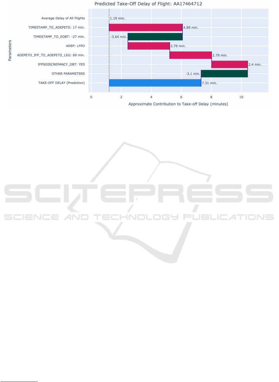
Figure 1: Example of explanation generated for a single instance of flight TOT delay prediction using LIME. The red and
green horizontal bars correspond to the contributions for increasing and decreasing the delay respectively, and the blue bar
corresponds to the predicted delay.
tree-ensemble classifiers. These studies are the
only notable ones found in the literature which
contributed to improving the interpretability of the
tree-ensemble models for classification tasks with
indications towards their use in regression tasks.
From the literature, it is evident that less effort
is given towards making the ensemble models
(e.g., XGBoost) interpretable for regression tasks.
Moreover, different state-of-the-art methods produce
explanations that differ in the contents of the output.
Under these circumstances, this study aims to
improve the interpretability of XGBoost by utilising
its mechanisms by design. The main contribution of
this study is twofold –
• Explaining the predictions of XGBoost regression
models using decision rules extracted from the
trained model.
• Generation of counterfactuals from the actual
neighbourhood of the test instance.
1.1 Motivation
The work presented in this paper is further motivated
by a real-world regression application for the aviation
industry. Particularly, the regression task is to predict
the flight take-off time (TOT) delay from historical
data to support the responsibilities of the Air Traffic
Controllers (ATCO). It is worth mentioning that the
aviation industry experiences a loss of approximately
100 Euros on average per minute for Air Traffic
Flow Management (ATFM) (Cook and Tanner, 2015).
The Federal Aviation Administration (FAA)
1
reported
in 2019 that the estimated cost due to delay,
1
https://www.faa.gov/
considering passengers, airlines, lost demand, and
indirect costs, was thirty-three billion dollars (Lukacs,
2020). The significant expenses provide the rationale
for increased attention towards predicting TOT and
reducing delays of flights (Dalmau et al., 2021).
To solve the problem of predicting flight TOT
delay, an interpretable system was developed to
incorporate the existing operational interface of the
ATCOs. In the process, the prediction model was
developed with XGBoost and its prediction was
made interpretable with the help of several popular
XAI tools, such as LIME – Local Interpretable
Model-agnostic Explanation. Qualitative evaluation
in the form of a user survey was conducted for the
developed system with the following scenario –
The current time is 0810 hrs. AFR141 is at the
gate and expected to take off from runway 09 at 0910
hrs. It is predicted that this flight will be delayed for
unknown minutes. After this, the aircraft has 2 more
flights in the day. Concurrently, SAS652 is in the last
flight leg of the day and is expected to land on runway
09 at 0916 hrs. Moreover, there is a scheduled runway
inspection at 0920 hrs.
The target users of the survey were the ATCOs,
both professionals and students. Participants were
prompted with several scenarios similar to the
scenario stated above and corresponding predictions
of the delay with explanation as illustrated in Figure 1,
which varied based on the explainability tool used to
generate the explanation. At the end of each scenario,
the participants were asked to respond to questions
to evaluate the effectiveness of the XAI methods in
explaining the prediction results.
The outcome of the user survey was deduced as–
the contribution to the final delay of the selected
ICAART 2024 - 16th International Conference on Agents and Artificial Intelligence
1346

features from the XAI methods would not impact
the operational relevance of the information received,
though the explanations are understandable. This
rationalisation was also reflected in the qualitative
interviews including the preference for user-centric
feature selection in the explanations and their
corresponding values on which the practitioners can
act to mitigate the issues of delays. Extensive details
on the presented use case can be found in a prior work
by the authors (Jmoona et al., 2023).
Based on the outcome of the previous study, the
aim was to generate a rule set and counterfactuals
in support of the prediction from XGBoost so that
the understanding of the operational relevance of the
selected features is improved. Particularly, XGBoost
is an ensemble of decision trees that are interpretable
by nature as the prediction rules from a single
decision tree are easily obtained (Gunning and Aha,
2019). This intrinsic characteristic of XGBoost
created the hypothesis of this work to extract decision
rules from the trained XGBoost model and generate
counterfactuals that suggest changes in the feature
values influencing the prediction.
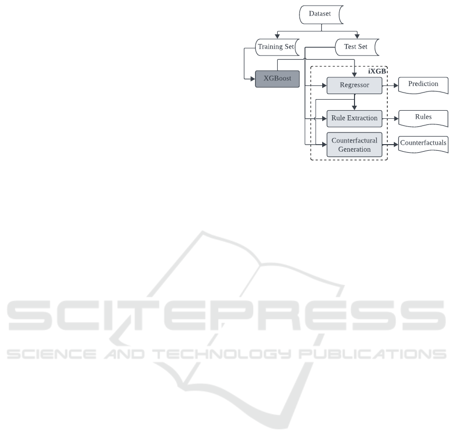
2 iXGB – INTERPRETABLE
XGBoost
The mechanism of the proposed iXGB is illustrated
in Figure 2, which utilises the trained XGBoost
regression model as the starting point. The principal
components of iXGB are the XGBoost regressor,
the rule extractor and the counterfactual generator.
Among these, the last two are described in the
following subsections including the formal definitions
from the context of a regression problem where the
first component is addressed.
2.1 Definitions
The regression model Ω is defined to predict a
continuous target variable y
i
∈ Y , based on a set
of m independent features or attributes a
1
, . . . , a
m
represented by the vector x
i
= [x
i1
, . . . , x
im
] and x
i
∈
X . The dataset consists of n observations, each
comprising a feature vector x
i
and its corresponding
target value y
i
, where i = 1, . . . , n. The objective of
the regression model is to learn a mapping function
f (x
i
) = ˆy
i
on (X
train
, Y
train
) that can accurately
estimate the target variable y
i
∈ Y
test
given the input
feature vector x
i
∈ X
test
. Here, the (X
train
, Y
train
) and
(X
test
, Y
test
) are the training and test sets respectively
split from the given dataset at a prescribed ratio.
iXGB
Dataset
Training Set Test Set
XGBoost
Regressor
Rule Extraction
Counterfactural
Generation
Prediction
Rules
Counterfactuals
Figure 2: Overview of the mechanism of the proposed
iXGB. The grey-coloured boxes with lighter shades depict
the principal components of iXGB.
In this study, Ω refers to an XGBoost (Chen
and Guestrin, 2016) regression model for which the
corresponding f computes the sum of residuals δ
from p decision trees d
k
, where k = 1, . . . , p and by
definition, δ
d
1
> δ
d
2
> · · · > δ
d
p
. Therefore, f is
formalised as –
f (x
i
) =
p
∑
k=1
δ
d
k
(1)
iXGB explains f (x
i
) as a pair of objects: hr, Φi,
where r = c → ˆy
i
describing f (x
i
) = ˆy
i
. Here, c
contains the conditions on the features a
1
, . . . , a
m
.
And, Φ is the set of counterfactuals. A counterfactual
is defined as an instance x
0
i
as close as possible to a
given x
i
with different values for at least one or more
features a, but for which f (x
i
) outputs a different
prediction ˆy
i
0
, i.e., y
i
6= ˆy
i
0
.
2.2 Extraction of Rules
The decision rules r supporting the prediction ˆy
i
by
the trained XGBoost regressor f is extracted from the
last trees (δ
d
p
) while regressor f predicts y for the q
closest neighbours of the instance x
i
. The intuition
behind using the last tree is that it generates the lowest
residual by definition of XGBoost. In other words,
the prediction is more accurate than the other trees
in f . The closest neighbours of x
i
are determined
using Euclidean distance metric. The value of q can
be determined by changing the value and observing
the quality of generated rules. Finally, all rules
from the decision paths of closest neighbours and x
i
are merged for each feature and the r is obtained.
The decision paths of the closest instances are also
included to obtain a generalised rule for the decision
region. Algorithm 1 presents the steps of extracting
rules with iXGB.
iXGB: Improving the Interpretability of XGBoost Using Decision Rules and Counterfactuals
1347

Algorithm 1: Rule Extraction.
Input: f : regressor, x
i
: test instance, X
test
: test
set, q: number of neighbours
Output: r: decision rule
1 CN = {cn
1
, . . . , cn
q
} ← q closest neighbours of
x
i
from X
test
within the its cluster
2 DP = {d p
x
i
, d p
cn
1
, . . . , d p
cn
q
} ← decision
paths from δ
d
p
of f for {x
i
} ∪CN
3 r ← merge the conditions from DP for each
feature a
j
, where j = 1, . . . , m
4 return r
2.3 Generation of Counterfactuals
The pseudo-code for generating counterfactuals is
stated in Algorithm 2. In the process of generating
the counterfactuals, all the instances of the test set
are clustered arbitrarily to form decision boundaries
around the instances based on their characteristics. In
this study, K-Means clustering is used and the number
of clusters is determined with the Elbow method
(Yuan and Yang, 2019). Then, the closest neighbours
of the test instance x
i
in other clusters than its own are
selected. The differences in the feature values and the
change in predicted values are calculated for x
i
versus
the closest neighbours. Lastly, the pairs of differences
in feature values and the changes in prediction are
generated as the set of counterfactuals Φ.
Algorithm 2: Counterfactual Generation.
Input: f : regressor, x
i
: test instance, X
test
: test
set, q: number of neighbours
Output: Φ: set of counterfactuals
1 C ← form arbitrary number of clusters with the
instances of X
test
2 CN
0
= {cn
0
1
, . . . , cn
0
q
} ← q closest neighbours
of x
i
in X
test
which are in different cluster than
x
i
, i.e., C(x
i
) 6= C(cn
0
j
), where j = 1, . . . , q
3 {∆A
1
, . . . , ∆A
q
} ← differences in the feature
values of x
i
and CN
0
4 {∆y
0
1
, . . . , ∆y
0
q
} ← differences in the predictions
with f for x
i
and CN
0
5 Φ ← {(∆A
1
, ∆y
0
1
), . . . , (∆A
q
, ∆y
0
q
)}
6 return Φ
3 MATERIALS AND METHODS
The implementation of iXGB was done using Python
scripts. Scikit–Learn (Pedregosa et al., 2011)
interface was used to build the models of XGBoost
regressor and K-Means clustering. The visualisations
were generated using Matplotlib (Hunter, 2007) and
Seaborn (Waskom, 2021). The datasets and metrics
used to evaluate the performance of iXGB are
discussed in the following subsections.
3.1 Datasets
Three different datasets were used in the conducted
experiments for this study. Among them, the first
one is the real-world dataset associated with the
motivating study described in Section 1.1, and the
other two are benchmark datasets. The summary of
the datasets is presented in Table 1 followed by brief
descriptions of the datasets below.
Table 1: Summary of the datasets used for evaluating the
performance of iXGB.
Dataset Features Instances
Flight Delay 5 1000
Auto MPG 7 392
Boston Housing 13 516
The real dataset was collected and processed by
EUROCONTROL
2
from the Enhanced Tactical Flow
Management System (ETFMS) flight data messages
containing all flights in Europe throughout the year
2019, from May to October. For this study, the
dataset was acquired from Aviation Data for Research
Repository
3
. The dataset consists of fundamental
details of the flights, flight status, preceding flight
legs, ATFM regulations, weather conditions, calendar
information, etc. The definitions of the features from
the dataset are described in the works of Koolen and
Coliban (2020) and Dalmau et al. (2021). Here,
the target variable is the flight take-off time delay
in minutes. The acquired dataset contained 42
features, whereas only 5 features were considered
for this study. The exclusion of the features was
done based on the observation of predicting flight
take-off delay from two different sets of data as
illustrated in Figure 3. In the figure, the prediction
performance of XGBoost improves until the top 5
most important features are used from the data. Here,
the feature importance values are obtained from the
global weights generated by XGBoost.
The benchmark datasets used in the experiments
are datasets commonly used to evaluate models
built for regression tasks. The first benchmark
dataset is the Auto MPG dataset (Quinlan, 1993)
2
https://www.eurocontrol.int/
3
https://www.eurocontrol.int/dashboard/rnd-data-
archive
ICAART 2024 - 16th International Conference on Agents and Artificial Intelligence
1348

Figure 3: Prediction Performance of XGBoost in terms of
MAE for flight delay prediction with different numbers of
features ranked by XGBoost feature importance from two
different subsets of the data.
containing information about various car models,
including attributes such as cylinders, displacement,
horsepower, weight, acceleration, model year, and
origin in numerical features. The target variable is the
miles per gallon, representing the fuel efficiency of
the cars. The other benchmark dataset was the Boston
Housing dataset (Harrison and Rubinfeld, 1978). It
contains both numerical and categorical features, such
as per capita crime rate, the average number of rooms
per dwelling, distance to employment centres, and
others. Here, the target variable is the median value
of owner-occupied homes, which is generally utilised
as a proxy for housing prices.
3.2 Metrics
The prediction performances of the models are
evaluated using Mean Absolute Error (MAE) and
standard deviation of the Absolute Error (σ
AE
).
MAE is the average difference between the actual
observation y
i
and the prediction ˆy
i
from the model.
σ
AE
signifies the dispersion of the absolute error
around the MAE. The measures were calculated using
Equations 2 and 3 respectively.
MAE =
1
n
n
∑
i=1
|
y
i
− ˆy
i
|
(2)
σ
AE
=
s
1
n
n
∑
i=1
(
|
y
i
− ˆy
i
|
− MAE)
2
(3)
To assess the quality of the extracted decision
rules, the metric coverage or support (Molnar, 2022)
was utilised. Coverage is the percentage of instances
from the dataset which follow the given set of rules.
It is calculated using the Equation 4 –
coverage =
|instances to which the rule applies|
|instances in the dataset|
(4)
4 EVALUATION AND RESULTS
The proposed approach was evaluated through a
series of experiments within the context of regression
problems. The experimental procedures and the result
of the evaluation experiments are presented in this
section.
To evaluate the extracted rules and the predictions
from iXGB, LIME (Ribeiro et al., 2016) is considered
as the baseline, which is widely used in recent
literature to generate rule-based explanations (Islam
et al., 2022). LIME is developed based on the
assumption that the behaviour of an instance can
be explained by fitting an interpretable model (e.g.,
linear regression) with a simplified representation
of the instance and its closest neighbours. While
predicting a single prediction of a black box model,
LIME generates an interpretable representation of
the input instance. In this step, it standardises the
input by modifying the values of the measurement
unit. The standardisation causes LIME to lose the
original proportion of values for regression. In the
next step, LIME perturbs the values of the simplified
input and predicts using the black box model, thus
generating the data on which the interpretable model
trains. Next, LIME draws samples from the generated
data based on their similarity to select the closest
neighbours. Lastly, a linear regression model is
trained with the sampled neighbours. With the
prediction from the linear regression model and the
value ranges from the neighbourhood, LIME presents
the local explanation with rules.
4.1 Prediction Performance
The first evaluation experiment was conducted to
assess the prediction performance of the proposed
approach. For each dataset described in Section
3.1, the MAE and σ
AE
were calculated using
Equations 2 and 3. For iXGB, the predictions remain
unchanged as the predictions are directly taken from
the XGBoost models which were compared with
the target values from the datasets. For LIME, the
predictions are compared with the predictions from
XGBoost and the target values from the datasets.
The results of all the calculations of MAE and σ
AE
are illustrated in Figure 4. For Boston Housing
and Flight Delay datasets, it is observed that the
error in prediction by iXGB is better than the LIME
predictions. However, for all the datasets, the
predictions from LIME are more erroneous than
iXGB when compared to the original target values
from the datasets. These observations advocate
that iXGB retains the prediction performance of the
iXGB: Improving the Interpretability of XGBoost Using Decision Rules and Counterfactuals
1349

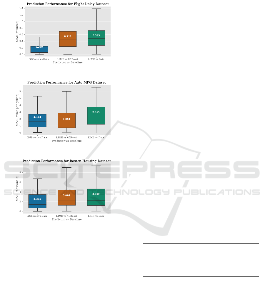
XGBoost regressor than the surrogate LIME.
(a) Flight Delay Dataset.
(b) Auto MPG Dataset.
(c) Boston Housing Dataset.
Figure 4: Comparison of prediction performance of
iXGB and LIME in terms of MAE with three different
datasets. Blue-coloured coloured box-plots are for
iXGB prediction compared with the target values. Red-
and green-coloured box-plots are for LIME predictions
compared with XGBoost prediction and the target values
respectively. The mean values are presented on the
corresponding box–plots.
By design, LIME perturbs the input values to
generate samples to train an interpretable model
(e.g., linear regression) and use that model for
generating the local explanations. However, the
literature prohibits modification of measurement units
for regression tasks since this operation destroys the
original proportion of the input values (Letzgus et al.,
2022). On the other hand, while explanations are
generated with iXGB, the prediction performance
of XGBoost is not compromised. Under these
circumstances, iXGB can be utilised by replacing
the surrogate models for rule-based explanation
(e.g., LIME) when performing regression tasks with
XGBoost.
4.2 Coverage of Decision Rule
To evaluate the quality of rules generated from iXGB,
they were compared with the rules extracted from
LIME. For simplicity, only the rules extracted for
a single instance of prediction from the Auto MPG
dataset by iXGB and LIME are presented. Using
Algorithm 1, the following rule (r) is extracted from
iXGB considering 5 closest instances from the test
set:
IF (cylinders < 4.00) AND
(displacement <= 74.50) AND
(horsepower >= 96.50) AND
(2305.00 <= weight < 2337.50) AND
(13.10 <= acceleration < 13.75) AND
(model_year <= 72.00) AND
(origin >= 3.00)
THEN (mpg = 19.00)
And, the decision rule extracted from LIME is:
IF (cylinders <= 4.00) AND
(displacement <= 98.00) AND
(88.00 < horsepower <= 120.00) AND
(2157.00 < weight <= 2672.00) AND
(acceleration <= 14.15) AND
(model_year <= 73.00) AND
(origin > 2.00)
THEN (mpg = 23.66)
Table 2: Coverage scores (average ± standard deviation)
of the rules extracted from iXGB and LIME. For local
explanation, lower values are better which are emphasised
with blue fonts.
Dataset
Coverage
iXGB LIME
Auto MPG 2.71 ± 1.55 7.24 ± 13.89
Boston Housing 2.53 ± 1.56 1.36 ± 0.87
Flight Delay 3.06 ± 1.41 20.50 ± 22.29
In both the decision rules, all the features from
the dataset are present. Particularly, for the feature
weight the value range is smaller in the rule extracted
from iXGB than the rule extracted from LIME. Again,
the conditions are different for the feature origin
but both the rules indicate values greater or equal to
3.00. While rules were generated considering all the
datasets, it was observed that the value ranges from
the rules extracted from iXGB are smaller than the
rules from LIME for the same instances.
ICAART 2024 - 16th International Conference on Agents and Artificial Intelligence
1350

Table 3: Sample set of counterfactuals generated using iXGB from the Auto MPG dataset.
Change in Feature Values
Change
in Target
cylinders displacement hp weight acceleration model year origin
+1 +43 -2 +42 +2 -2 0 -50%
0 -27 23 -29 -4 -3 +2 -10%
0 -27 +23 -29 -4 -3 +2 -10%
0 +5 +20 +22 -2 -11 0 +20%
0 +15 +30 -8 -6 -11 +2 +45%
0 -22 +11 -13 +2 -11 +2 +75%
0 -27 +23 -36 -4 -1 +2 +90%
Table 4: Sample set of counterfactuals generated using iXGB from the Boston Housing dataset.
Change in Feature Values
Change
in Target
crim zn indus chas nox rm age dis rad tax prratio blck lstat
+1 0 0 0 0 +1 [phone] +3 -600%
[phone] +9 -275%
+7 0 0 0 0 0 +5 0 0 0 0 -83 +6 -200%
-1 0 0 0 0 0 +4 0 0 0 0 -33 +5 +40%
+1 0 0 0 0 0 [phone] +8 +50%
Furthermore, the coverage of the rules from
iXGB and LIME were calculated using Equation
4. The results for all the datasets are presented
in Table 2. The coverage values of rules for
classification models are expected to be higher for
better generalisation (Guidotti et al., 2019). In
the case of local interpretability, the rule needs to
define a single instance of prediction that is the
opposite of generalisation (Ribeiro et al., 2018).
This claim is also supported in the works of (Sagi
and Rokach, 2021). The authors argued that the
tree-ensemble models create several trees to improve
the performance of the model resulting in lots of
decision rules for prediction. This mechanism makes
it harder to be understood by the end users. Thus, the
smaller coverage values are considered better in this
evaluation.
4.3 Counterfactuals
For all the datasets, the sets of counterfactuals
(Φ) were generated by selecting a random instance
from the test set to assess the impact on the target
when the feature values are changed. The process
described in Algorithm 2 was followed to generate
the counterfactuals. Here, the counterfactuals are the
instances around the boundary of the closest clusters
of the selected instance. The number of clusters
was chosen with the Elbow method (Yuan and Yang,
2019), which was 7 for the Auto MPG dataset and 5
for both Boston Housing and Flight Delay datasets.
Unlike, counterfactuals from a classification task,
the boundaries of the clusters formed with the test
instances can be referred to as decision boundaries as
they are clustered based on the characteristics of the
data.
The sample set of counterfactuals from the Auto
MPG dataset is presented in Table 3. For the table,
it is found that the target value changes when all
the feature values are changed except the feature
cylinders in the first counterfactual. Likewise, for the
Boston Housing dataset (Table 4), 8 out of 13 features
needed not be changed to find the counterfactuals.
Again, changing the values of only 3 features can
decrease the target value by 275%. Lastly, the
counterfactuals from the Flight Delay dataset are
presented in Table 5 which can be interpreted in a
similar way to the last two tables. For all the tables
with counterfactuals, the feature names are shown as
it is present in the dataset since the names are not
directly subjected to the mechanism of the proposed
iXGB.
The set of counterfactuals for any regression task
can support the end users when they need to modify
some feature values to achieve any target. Such
question can be – what would it take to increase
the target value by some percentage?. However,
the change can be measured both in percentage and
absolute values. After all, the counterfactuals would
facilitate the decision-making process of end users by
iXGB: Improving the Interpretability of XGBoost Using Decision Rules and Counterfactuals
1351

Table 5: Sample set of counterfactuals generated using iXGB from the Flight Delay dataset.
Change in Feature Values
Change
in Target
ts leg to ts flight duration leg ts to ta leg ta leg ts ifp to ts
-118 -56 +9 +4 +3 -10%
+2 +2 +2 +2 +2 -5%
-14 +7 +11 -36 -89 -5%
-21 +35 +25 -5 -34 +5%
+29 +46 -25 -8 -49 +5%
maintaining operational relevance.
5 CONCLUSION AND FUTURE
WORKS
XGBoost is widely adopted in regression tasks
because of its higher accuracy than other tree-based
ML models with the cost of interpretability.
Generally, the interpretability is induced to XGBoost
through using various XAI methods. These XAI
methods (e.g., LIME) rely on perturbed samples
to provide explanations for XGBoost predictions.
In this paper, iXGB is proposed by utilising the
internal structure of XGBoost to generate rule-based
explanations and counterfactuals from the same data
on which the model trains for prediction tasks. The
proposed approach is functionally evaluated on three
different datasets in terms of local accuracy and
quality of the rules, which shows the ability of
iXGB to improve the interpretability of XGBoost
reasonably. Future research directions include
theoretically grounded evaluation of the proposed
approach on more diverse datasets and different
real-world problems. Moreover, further investigations
are also required to adopt the proposed iXGB for
binary and multi-class classification tasks.
ACKNOWLEDGEMENTS
This study was supported by the following projects;
i) ARTIMATION (Transparent Artificial intelligence
and Automation to Air Traffic Management Systems),
funded by the SESAR JU under the European Union’s
Horizon 2020 Research and Innovation programme
(Grant Agreement No. 894238) and ii) xApp
(Explainable AI for Industrial Applications), funded
by the VINNOVA (Sweden’s Innovation Agency)
(Diary No. 2021-03971).
REFERENCES
Blanchart, P. (2021). An Exact
Counterfactual-Example-based Approach to
Tree-ensemble Models Interpretability. ArXiv,
(arXiv:2105.14820v1 [cs.LG]).
Breiman, L. (2001). Random Forests. Machine Learning,
45(1):5–32.
Chen, T. and Guestrin, C. (2016). XGBoost: A Scalable
Tree Boosting System. In Proceedings of the 22nd
ACM SIGKDD International Conference on Knowledge
Discovery and Data Mining, pages 785–794, San
Francisco California USA. ACM.
Cook, A. J. and Tanner, G. (2015). European Airline Delay
Cost Reference Values. Technical report, University of
Westminster, London, UK.
Dalmau, R., Ballerini, F., Naessens, H., Belkoura, S., and
Wangnick, S. (2021). An Explainable Machine Learning
Approach to Improve Take-off Time Predictions. Journal
of Air Transport Management, 95:102090.
Friedman, J. H. (2001). Greedy Function Approximation:
A Gradient Boosting Machine. The Annals of Statistics,
29(5).
Guidotti, R., Monreale, A., Giannotti, F., Pedreschi, D.,
Ruggieri, S., and Turini, F. (2019). Factual and
Counterfactual Explanations for Black Box Decision
Making. IEEE Intelligent Systems, 34(6):14–23.
Gunning, D. and Aha, D. W. (2019). DARPA’s
Explainable Artificial Intelligence Program. AI
Magazine, 40(2):44–58.
Hara, S. and Hayashi, K. (2016). Making Tree Ensembles
Interpretable. ArXiv, (arXiv:1606.05390v1 [stat.ML]).
Harrison, D. and Rubinfeld, D. L. (1978). Hedonic
Housing Prices and the Demand for Clean Air.
Journal of Environmental Economics and Management,
5(1):81–102.
Hunter, J. D. (2007). Matplotlib: A 2D Graphics
Environment. Computing in Science & Engineering,
9(3):90–95.
Islam, M. R., Ahmed, M. U., Barua, S., and Begum, S.
(2022). A Systematic Review of Explainable Artificial
Intelligence in Terms of Different Application Domains
and Tasks. Applied Sciences, 12(3):1353.
Jmoona, W., Ahmed, M. U., Islam, M. R., Barua, S.,
ICAART 2024 - 16th International Conference on Agents and Artificial Intelligence
1352

Begum, S., Ferreira, A., and Cavagnetto, N. (2023).
Explaining the Unexplainable: Role of XAI for Flight
Take-Off Time Delay Prediction. In Maglogiannis, I.,
Iliadis, L., MacIntyre, J., and Dominguez, M., editors,
Artificial Intelligence Applications and Innovations –
AIAI 2023, volume 676, pages 81–93, L
´
eon, Spain.
Springer Nature Switzerland.
Koolen, H. and Coliban, I. (2020). Flight
Progress Messages Document. Technical report,
EUROCONTROL, Brussels, Belgium.
Letzgus, S., Wagner, P., Lederer, J., Samek, W., Muller,
K.-R., and Montavon, G. (2022). Toward Explainable
Artificial Intelligence for Regression Models: A
methodological perspective. IEEE Signal Processing
Magazine, 39(4):40–58.
Lukacs, M. (2020). Cost of Delay Estimates. Technical
report, Federal Aviation Administration, Washington,
DC, USA.
Molnar, C. (2022). Interpretable Machine Learning:
A Guide for Making Black Box Models Explainable.
Christoph Molnar, Munich, Germany, 2nd edition.
Nalenz, M. and Augustin, T. (2022). Compressed Rule
Ensemble Learning. In Proceedings of The 25th
International Conference on Artificial Intelligence and
Statistics, pages 9998–10014. PMLR.
Pedregosa, F., Varoquaux, G., Gramfort, A., Michel, V.,
Thirion, B., Grisel, O., Blondel, M., Prettenhofer,
P., Weiss, R., Dubourg, V., Vanderplas, J., Passos,
A., Cournapeau, D., Brucher, M., Perrot, M., and
Duchesnay,
´
E. (2011). Scikit-learn: Machine Learning
in Python. Journal of Machine Learning Research,
12(85):2825–2830.
Quinlan, J. R. (1993). Combining Instance-based and
Model-based Learning. In Proceedings of the Tenth
International Conference on International Conference
on Machine Learning (ICML 1993), pages 236–243,
Amherst, MA, USA. Morgan Kaufmann Publishers Inc.
Ribeiro, M. T., Singh, S., and Guestrin, C. (2016). “Why
Should I Trust You?”: Explaining the Predictions of Any
Classifier. In Proceedings of the 22nd ACM SIGKDD
International Conference on Knowledge Discovery and
Data Mining (KDD 2016), pages 1135–1144, San
Francisco, CA, USA. ACM.
Ribeiro, M. T., Singh, S., and Guestrin, C. (2018).
Anchors: High-Precision Model-Agnostic Explanations.
In Proceedings of the AAAI Conference on Artificial
Intelligence, volume 32.
Sagi, O. and Rokach, L. (2021). Approximating XGBoost
with an interpretable decision tree. Information Sciences,
572:522–542.
Waskom, M. (2021). Seaborn: Statistical Data
Visualization. Journal of Open Source Software,
6(60):3021.
Yuan, C. and Yang, H. (2019). Research on K-Value
Selection Method of K-Means Clustering Algorithm. J,
2(2):226–235.
iXGB: Improving the Interpretability of XGBoost Using Decision Rules and Counterfactuals
1353