A Mutual Information Based Discretization-Selection Technique

Artur J. Ferreira

1,3 a

and M

ario A. T. Figueiredo

2,3 b

ISEL, Instituto Superior de Engenharia de Lisboa, Instituto Polit

ecnico de Lisboa, Portugal

IST, Instituto Superior T

ecnico, Universidade de Lisboa, Portugal

Instituto de Telecomunicac¸

oes, Lisboa, Portugal

ﬁ

Keywords:

Bit Allocation, Classiﬁcation, Explainability, Feature Discretization, Feature Selection, Machine Learning,

Mutual Information, Supervised Learning.

Abstract:

In machine learning (ML) and data mining (DM) one often has to resort to data pre-processing techniques to

achieve adequate data representations. Among these techniques, we ﬁnd feature discretization (FD) and fea-

ture selection (FS), with many available methods for each one. The use of FD and FS techniques improves the

data representation for ML and DM tasks. However, these techniques are usually applied in an independent

way, that is, we may use a FD technique but not a FS technique or the opposite case. Using both FD and FS

techniques in sequence, may not produce the most adequate results. In this paper, we propose a supervised

discretization-selection technique; the discretization step is done in an incremental approach and keeps infor-

mation regarding the features and the number of bits allocated per feature. Then, we apply a selection criterion

based upon the discretization bins, yielding a discretized and dimensionality reduced dataset. We evaluate our

technique on different types of data and in most cases the discretized and reduced version of the data is the

most suited version, achieving better classiﬁcation performance, as compared to the use of the original fea-

tures.

1 INTRODUCTION

In machine learning (ML) and data mining (DM)

when dealing with large amounts of data, one may

need to apply data pre-processing methods to obtain a

more suitable representation (Ram

ırez-Gallego et al.,

2017). For the data pre-processing stage, there are

many available techniques, among which we ﬁnd fea-

ture discretization (FD) and feature selection (FS)

techniques (Duda et al., 2001; Guyon et al., 2006;

Guyon and Elisseeff, 2003).

Both FD and FS are vast research ﬁelds with

many techniques available in the literature. How-

ever, many efforts continue to be developed on those

ﬁelds (Alipoor et al., 2022; Chamlal et al., 2022;

Huynh-Cam et al., 2022; Jeon and Hwang, 2023).

Learning on high-dimensional (HD) data is a chal-

lenge, due to the curse of dimensionality (Bishop,

1995), which poses many difﬁculties to the problem

of ﬁnding the best features and their best represen-

tation, among a large set of features. It is known

from the literature that the use of FD and FS im-

https://orcid.org/0000-0002-6508-0932

https://orcid.org/0000-0002-0970-7745

proves the performance of ML and DM tasks (Witten

et al., 2016). Often, researchers develop independent

FD or FS techniques without addressing their joint or

combined use. However, it is expected that an ade-

quate combination of discretization and selection pro-

cedures would provide better results than the indepen-

dent use of these techniques.

In this paper, we propose the mutual information

discretization-selection (MIDS) algorithm, which is a

hybrid discretization-selection technique. An FS ﬁl-

ter is applied on the discretized data, guided by the

discretization stage details, yielding a discretized and

reduced dataset suitable for learning. The variable

number of discretization bins assigned to each fea-

ture provides a hint on the explainability and on the

importance of each feature.

The remainder of this paper is organized as fol-

lows. In Section 2, we overview related work and

techniques for FS and FD. The proposed approach

and its key insights are described in Section 3. The

experimental evaluation procedure is reported in Sec-

tion 4. Finally, Section 5 ends the paper with conclud-

ing remarks and directions of future work.

436

Ferreira, A. and Figueiredo, M.

A Mutual Information Based Discretization-Selection Technique.

DOI: 10.5220/0012467300003654

Paper published under CC license (CC BY-NC-ND 4.0)

In Proceedings of the 13th International Conference on Pattern Recognition Applications and Methods (ICPRAM 2024), pages 436-443

ISBN: 978-989-758-684-2; ISSN: 2184-4313

2 RELATED WORK

We brieﬂy review some related work regarding key

aspects of FS and FD techniques over the past years.

In Section 2.1, we describe the key notation fol-

lowed in this paper. Section 2.2 overviews the use of

FS techniques with emphasis on ﬁlter techniques ad-

dressed in the experimental evaluation. Finally, Sec-

tion 2.3 overviews FD techniques with some details

about the techniques considered in this work.

2.1 Notation and Terminology

In this paper, we use the following terminology. Let

X = {x

, . . . , x

} be a dataset, with n patterns. Each

pattern denoted as x

is a d−dimensional vector, with

d being the number of features. Each dataset X is

represented by a n × d matrix; the rows hold the pat-

terns, while the columns are the features, denoted as

. We denote the number of distinct class labels as C,

with c

∈ {1, . . . ,C} being the class of pattern i and

y = {c

, . . . , c

} is the set of class labels.

2.2 Feature Selection

FS techniques bring many beneﬁts to ML and DM

tasks, the accuracy of a classiﬁer is often improved

mitigating the effects of the curse of dimensionality

and training is faster (Guyon et al., 2006; Guyon and

Elisseeff, 2003). Over the past years, many different

FS algorithms have been proposed. These algorithms

are usually placed into one of four categories: ﬁlter,

wrapper, embedded, and hybrid.

Filter methods check the adequacy of a feature

subset using characteristics of that subset, without

resorting to any learning algorithm and keep some

of the features, discarding others. Thus, ﬁlter ap-

proaches are agnostic in the sense that they do not re-

sort to any learning algorithm. In some big-data and

high-dimensional datasets, ﬁlters are often the only

suitable category of FS methods to be used. One

of the most successful ﬁlters is the fast correlation-

based ﬁlter (FCBF), under the relevance-redundancy

(RR) framework for the FS task (Yu and Liu, 2004).

FCBF computes the feature-class and feature-feature

association. It selects a set of features highly related

with the class. In the ﬁrst step, these features are

called predominant and the correlation is assessed by

the symmetrical uncertainty (SU), deﬁned as

SU(U,V ) =

2MI(U;V )

H(U) + H(V)

, (1)

where H denotes the Shannon entropy and MI denotes

the mutual information (MI) (Cover and Thomas,

2006), where U and V are feature vectors or class la-

bel vectors. SU is zero for independent random vari-

ables and one for deterministically dependent random

variables. In the second step, a redundancy detection

procedure ﬁnds redundant features among the pre-

dominant ones. These redundant features are further

split, keeping the ones that are the most relevant to

the class. For recent surveys on FS techniques, please

see (Pudjihartono et al., 2022; Dhal and Azad, 2022).

2.3 Feature Discretization

FD is a research ﬁeld with many available unsuper-

vised and supervised techniques, following different

criteria. We brieﬂy review some aspects of FD meth-

ods with emphasis on supervised techniques.

Many datasets have real-valued features; however,

some classiﬁcation algorithms can only deal with dis-

crete/categorical features, and for this reason a dis-

cretization procedure is necessary. FD techniques aim

at ﬁnding a representation of each feature that con-

tains enough information for the learning task at hand,

while ignoring minor ﬂuctuations that may be irrele-

vant for that task. In a nutshell, FD seeks more com-

pact and better representations of the data for learning

purposes. As a consequence, these discrete features

usually lead to both better accuracy and lower train-

ing time, as compared to the use of the original fea-

tures (Dougherty et al., 1995; Biba et al., 2007; Tsai

et al., 2008; Garc

ıa et al., 2013; Witten et al., 2016;

Ram

ırez-Gallego et al., 2017). Supervised FD ap-

proaches use class label information to compute the

cut-points in the discretization process.

The information entropy maximization (IEM)

method (Fayyad and Irani, 1993) is one of the old-

est and most used FD techniques. It assumes that the

most informative features to discretize are the most

compressible ones, which is an entropy minimization

heuristic. It works in a recursive approach computing

the discretization cut-points in such a way that it min-

imizes the number of bits to represent each feature.

The static class-attribute interdependence maxi-

mization (CAIM) algorithm (Kurgan and Cios, 2004)

aims to maximize the class-attribute interdependence

and to generate a (possibly) minimal number of dis-

crete intervals.

The class-attribute contingency coefﬁcient

(CACC) (Tsai et al., 2008) is based on the maximiza-

tion of a modiﬁcation of the contingency coefﬁcient,

overcoming the key drawbacks of earlier schemes

such as CAIM.

The mutual information discretization (MID) al-

gorithm was proposed by Ferreira and Figueiredo

(2013). It performs supervised FD with q bits per fea-

A Mutual Information Based Discretization-Selection Technique

437

ture, based on the assessment of the MI between the

discretized feature and the class label vector y. MID

searches for discretization intervals such that the re-

sulting discrete feature has the highest MI as possible

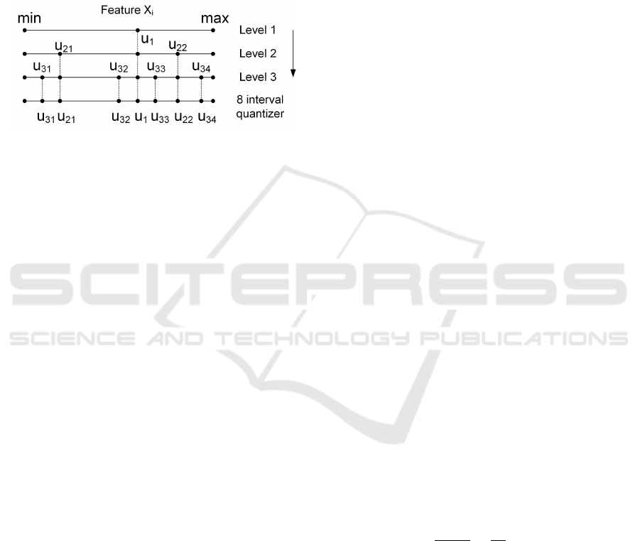
with the class label vector. Each feature is discretized

individually, by successively breaking its range of val-

ues into intervals with boundaries u

i j

, as depicted in

Figure 1 for a given feature, say X

, with q = 3 bits

(8-intervals), yielding the discretized feature

Figure 1: Mutual Information Discretization (MID) of one

feature with q = 3 bits, for a 8-interval discretized feature,

proposed by Ferreira and Figueiredo (2013).

The maximum value for MI(

;y) depends on

both the number of bits used to discretize X

and

the number of classes C. If we discretize X

with b

bits, its maximum entropy is H

max

(

) = b

bit/symbol; the maximum value of the class entropy

is H

max

(y) = log

to C equiprobable classes. Thus, the maximum value

of the MI between the class label and a discretized

feature (with b

bits) is upper bounded as

max{MI

(

;y)

} ≤ min{b

, log

(C)}. (2)

To ensure that the discretization process attains the

maximum possible value for the MI, one must choose

the maximum number of bits q following this expres-

sion. Thus, we have q ≥ ⌈log

(C)⌉, where ⌈.⌉ is the

ceiling operator.

3 PROPOSED APPROACH

In this section, we describe the key ideas of our ap-

proach and present them with an algorithm in Sec-

tion 3.1. We also show some insights on the dis-

cretization behavior for different datasets, in Sec-

tion 3.2.

3.1 Key Ideas and Algorithms

First, we state the key ideas of our proposal and then

we present it in an algorithmic style. For a dataset,

with n instances and d features, we use a static dis-

cretizer @disc, a relevance function @rel, and a fea-

ture selection technique @ f s, as follows:

• Use of the static discretizer @disc technique over

the training data, with an increasing number of

bits per feature.

• Discretize each feature starting with one bit (a bi-

nary feature) up to a maximum number of bits.

• For each feature, ﬁnd the minimum number of bits

such that maximizes @rel between the discretized

feature and the class label vector.

• For each feature, obtain its discretized version

with the minimum number of bits.

• Apply a feature selection technique @ f s on the

discretized features, resorting to the discretization

information.

We use the MID algorithm as @disc and @rel as

the MI between the discretized feature vector and the

class label vector. Algorithm 1 presents our proposal,

named as mutual information discretization-selection

(MIDS).

After using MIDS on a training set, we get a dis-

cretized and dimensionality reduced version. On the

FS procedure @ f s, we use ﬁlter techniques, namely:

• A relevance-based approach, which we denote as

MIDS, for simplicity.

• A relevance-redundancy approach, denoted as

MIDSred, performing a redundancy analysis af-

ter the discretization step.

On the relevance-based approach, we use a thresh-

old parameter to select the top-m features, from the

original set of d discretized features. We use a cu-

mulative relevance (CR) criterion as follows. Let

, ..., r

be the sorted relevance values and

∑

f =1

, (3)

be the CR of the top l most relevant features. We

select the number of features as the lowest value m

that satisﬁes the condition

∑

f =1

∑

i=1

≥ T

, (4)

where T

is a threshold (e.g., 0.95), leading to a frac-

tion of the top-m ranked features. The relevance is

the MI value computed on the discretization stage.

On the relevance-redundancy approach, we follow the

ideas by Ferreira and Figueiredo (2012). After com-

puting the sorted relevance values, we assess the re-

dundancy between the most relevant features. At the

end, we keep features with high relevance and low re-

dundancy, below some threshold, named as maximum

ICPRAM 2024 - 13th International Conference on Pattern Recognition Applications and Methods

438

Algorithm 1: Supervised mutual information discretization-selection (MIDS).

Input: X, n patterns of a d-dimensional training set.

y, n-length vector with class labels.

, the maximum number of bits per feature.

@ f s, a feature selection procedure.

Output:

′

, the discrete and reduced training set with n patterns and m dimensions.

, ..., Q

, set of m quantizers (one per feature).

b, m-length vector with the number of bits per feature.

1: For all features X

, with i ∈ {1, . . . , d}, compute their q

discretized versions with q bits per feature, with q ∈ {1, . . . , q

using MID as described in Figure 1.

2: Compute the MI matrix, M, with dimensions q

× d. Each element of M, denoted as M

, holds the MI between feature

discretized with j bits, and the class label vector y.

3: For each feature, identify the minimum number of bits that yields the maximum MI, denoted as b

. For each column of

M, locate the ﬁrst row (from top to bottom) that achieves the maximum MI. Create a d-dimensional vector b with the

minimum number of bits per feature, b

4: Quantize each feature X

using MID with b

bits,

= Q

5: Apply the FS procedure @ f s to

X, reducing its dimensionality from d to m, yielding

′

6: Return the discretized/reduced training set

′

, the quantizers Q

, and the vector with the number of bits per feature b.

similarity (M

). The redundancy is assessed with the

MI between two feature vectors.

3.2 Discretization Analysis

We now observe the contents of the M matrix deﬁned

in Algorithm 1. Figure 2 shows the increase of the

MI between each feature X

and the class label vec-

tor y, as a function of the number of bits per fea-

ture, q ∈ {1, . . . , 6}, for the Wine dataset with d = 13

features and C = 3 distinct labels. On the left-hand-

side, we have an image with the MI value with a color

scale; the image rows are the number of bits per fea-

ture q and the columns correspond to the d features.

For most features, we have an increment on the MI

value, as we increase q, stopping at some point. For

feature number 7, we observe a clear increase on the

MI when discretizing up to 4 bits. For feature number

3, we have the opposite behavior, with no increase on

the MI, regardless of the increase in q. On the right-

hand-side, the top plot shows the maximum MI after

discretization and the bottom plot exhibits the mini-

mum number of bits that yields maximum MI; no fea-

ture requires more than 4 bits and most features use 3

bits. There is a large variability on the MI values for

all the features.

Figure 3, left-hand-side, shows the histogram of

the ﬁnal MI values after discretization. On the right-

hand-side, we display the histogram of the b vector

elements. This assessment is done with the Colon

dataset with d = 2000 features and C = 2 distinct la-

bels. The MI values range from 0.0103 to 0.5954,

with a peak located around 0.1. Requiring 1, 2, 3, and

4 bits per feature, we have 86, 1134, 761, and 19 fea-

tures, respectively. No feature requires more than 4

bits for discretization.

We now check for the association between the

highest MI values and the minimum number of bits

per feature, in vector b, using scatter plots. Figure 4

depicts the value of MI as a function of the number

of bits per feature, for the Wine and Colon datasets,

with up to q = 6 bits per feature. No feature requires

more than 4 bits. There is no strong correlation be-

tween the MI value and the number of bits per fea-

ture. We have many features that achieve a high value

of MI with q = 1. Other features achieve higher MI

with q = 3 than with q = 4, which means that 3 bits is

sufﬁcient to achieve the maximum MI implying that

many features achieve their highest MI value with a

small number of bits.

4 EXPERIMENTAL EVALUATION

We now report the evaluation of our method. Sec-

tion 4.1 describes the datasets as well as the evalua-

tion metrics. In Section 4.2, we check the MIDS bit

allocation and compare it with other FD algorithms.

In Section 4.3, we check for the sensitivity of MIDS

with its input parameters. A FS assessment is pro-

vided in Section 4.4. Finally, Section 4.5 discusses

the ﬁndings of the experimental evaluation.

4.1 Datasets and Evaluation Metrics

Table 1 presents the datasets used in this work, with

different problems and diverse types of data. The

datasets are available at public repositories such as

University of California at Irvine (UCI) https://arch

A Mutual Information Based Discretization-Selection Technique

439

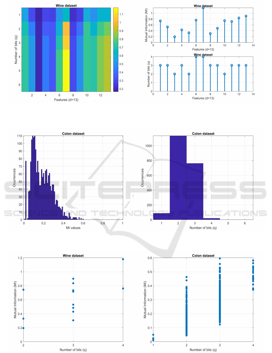
Figure 2: Discretization of the Wine dataset. Left: MI as a color scale image for the d = 13 features (image columns), as

functions of the number of bits per feature, q ∈ {1, . . . , 6} (image rows). Right: on top, the maximum MI between each

discretized feature and the class label vector; on bottom, the minimum number of bits that achieves the maximum MI.

Figure 3: Discretization of the Colon dataset. Left: histogram of the maximum MI values attained for the d = 2000 features.

Right: histogram of the number of bits allocated per feature.

Figure 4: Discretization of the Wine (left) and Colon (right) datasets. Scatter plot showing the MI value on the yy-axis as a

function of the number of bits per feature on the xx-axis.

ICPRAM 2024 - 13th International Conference on Pattern Recognition Applications and Methods

440

ive.ics.uci.edu/ml/index.php, the knowledge extrac-

tion evolutionary learning (KEEL), https://sci2s.ugr.

es/keel/datasets.php, and the ones available at https:

//csse.szu.edu.cn/staff/zhuzx/Datasets.html and https:

//jundongl.github.io/scikit-feature/datasets.html.

We report the test set error rate of 10-fold cross

validation for classiﬁcation with the linear support

vector machines (SVM) classiﬁer from Waikato en-

vironment for knowledge analysis (WEKA) (Frank

et al., 2016).

4.2 Bit Allocation per Feature

We assess the number of bits allocated to each feature

by the MIDS algorithm, setting T

= 1, that is, using

only discretization without performing feature selec-

tion. We aim to identify, for each dataset, the number

of bits allocated to each feature and the test error rate

of MIDS, compared with the original features and the

features discretized by the IEM, CAIM, and CACC

methods. Table 2 reports these results.

For most datasets, we observe that discretization

stops at q = 4 bits. Many datasets end up with many

features discretized with one bit; this may imply that

for these features it is mostly important if they are

present or absent (based on a given threshold), regard-

less of their exact value. The majority of features is

discretized with 2, 3, or 4 bits.

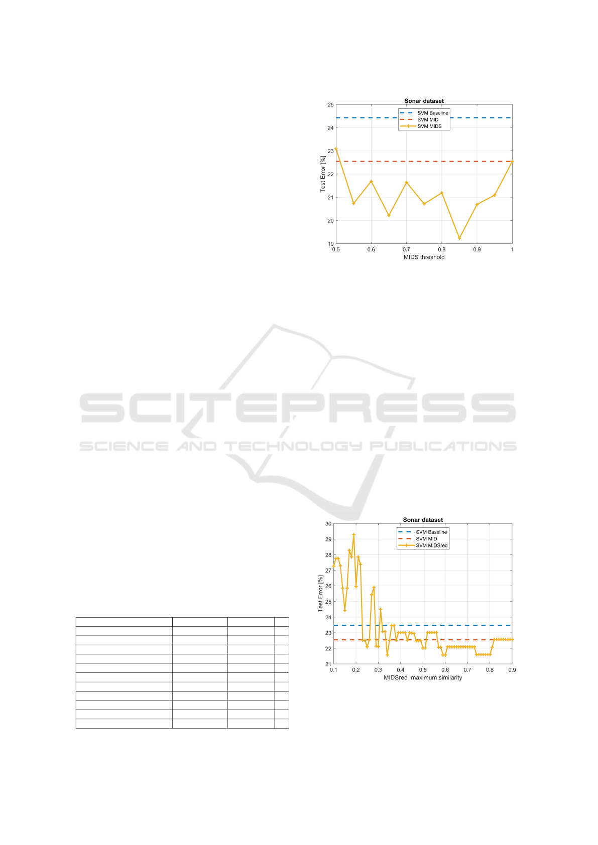
4.3 MIDS Parameter Sensitivity

We analyze the sensitivity of MIDS with the thresh-

old T

, for a ﬁxed number of bits per feature. Figure 5

shows the test set error rate (10-fold CV), as a func-

tion of the T

parameter ranging from 0.5 to 1, with

q = 4, for the Sonar dataset, with the SVM classiﬁer.

For this dataset, the optimal threshold value is

= 0.95, which yields the lowest error rate. We also

analyze how MIDSred behaves as a function of its

Table 1: Datasets with n instances (per class), d features

(numeric + nominal), and C classes.

∗

For the Dermatol-

ogy, SRBCT, and Wine datasets, the instance distribution

per class is 358 = 111 + 60 + 71 + 48 + 48 + 20, 83 =

29 + 25 + 11 + 18, and 178 = 59 + 71 + 48.

Dataset name and task n d C

Australian - credit card 690

(307+383)

(8+6)

Basehock - text classiﬁcation 1993

(994+999)

4862

(4862+0)

Colon - cancer detection 62

(22+40)

2000

(2000+0)

Dermatology - skin disease 358

∗

(34+0)

DLBCL - cancer detection 77

(58+19)

5469

(5469+0)

Heart - coronary disease 270

(150+120)

(13+0)

Hepatitis - detection 155

(123+32)

(19+0)

Spambase - email spam 4601

(2788+1813)

(54+0)

Sonar - signals 208

(97+111)

(60+0)

SRBCT - cancer detection 83

∗

2308

(2308+0)

Wine - cultivar classiﬁcation 178

∗

(13+0)

Figure 5: Test set error rate (10-fold CV) for the SVM clas-

siﬁer, on the Sonar dataset, with the original features, MIDS

(q = 4, T

= 1, no feature selection), and MIDS (q = 4 and

ranging from 0.5 to 1).

maximum similarity parameter, M

, for a ﬁxed num-

ber of bits per feature. Figure 6 shows the test set

error rate (10-fold CV), as a function of the M

pa-

rameter ranging from 0.1 to 0.9, with q = 4, for the

Sonar dataset, with the SVM classiﬁer. We ﬁnd that

the optimal maximum similarity value is in the range

from 0.57 to 0.81, achieving the lowest error rate.

4.4 Discretization and Selection

We now report the experimental results regarding the

test set error rate for 10-fold CV, after feature dis-

cretization and selection with MIDS and MIDSred,

on Table 3, with the SVM classiﬁer. We also ap-

ply the FCBF ﬁlter over the original and the dis-

cretized/selected data representation, to have a bench-

Figure 6: Test set error rate (10-fold CV) for the SVM clas-

siﬁer, on the Sonar dataset, with the original features, MIDS

(q = 4, T

= 1, no feature selection), and MIDSred (q = 4

and M

ranging from 0.1 to 0.9).

A Mutual Information Based Discretization-Selection Technique

441

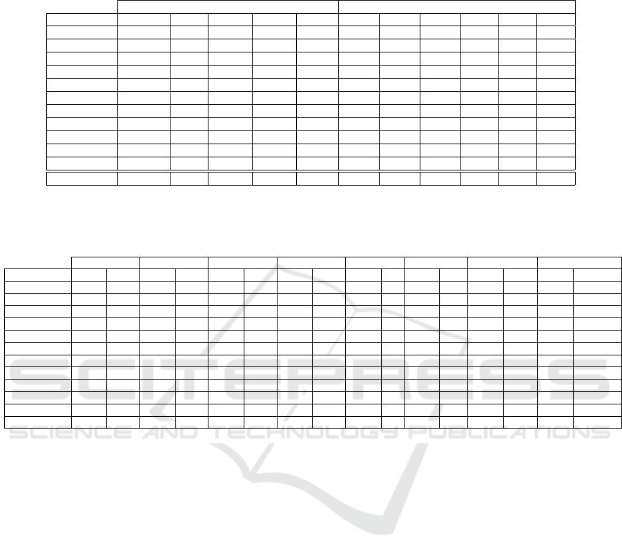
Table 2: The average test error rate (%) with the linear SVM classiﬁer with 10-fold CV, for the original features and the IEM,

CAIM, CACC, and MIDS discretized features. For MIDS we use T

= 1 (no FS) and we report the histogram of the number

of bits allocated to each feature, on the 10 folds, with q ∈ {1, . . . , 6}. The best result (lower error rate) is in boldface.

Error rate MIDS (T

= 1) allocated bits

Dataset Baseline IEM CAIM CACC MIDS q = 1 q = 2 q = 3 q = 4 q = 5 q = 6

Australian 14.49 14.49 44.49 14.49 14.49 69 33 25 13 0 0

Basehock 4.06 2.16 1.96 1.51 2.16 46408 2198 14 0 0 0

Colon 15.71 22.62 17.62 16.19 16.43 1029 11408 7403 160 0 0

Dermatology 2.23 2.52 5.31 2.23 1.39 330 0 10 0 0 0

DLBCL 2.50 5.18 5.18 2.50 2.50 4234 30421 19686 349 0 0

Heart 16.30 15.56 22.59 16.30 15.19 80 15 30 5 0 0

Hepatitis 19.88 18.54 19.83 19.83 16.63 132 27 26 5 0 0

Spambase 10.11 6.41 6.67 6.50 6.39 83 189 212 56 0 0

Sonar 22.12 21.12 22.10 21.64 16.31 18 181 339 62 0 0

SRBCT 0.00 0.00 1.25 1.25 0.00 73 3057 14531 5410 9 0

Wine 1.14 3.37 2.25 2.84 1.70 0 26 84 20 0 0

Average 9.86 10.17 13.56 9.57 8.47 - - - - - -

Table 3: The average test error rate (Err, %) and the average number of features (m) with the linear SVM classiﬁer with 10-fold

CV, using the original features, MID discretization, MIDS discretization/selection, and MIDSred discretization/selection. We

also apply the FCBF ﬁlter over the original and discretized data. The best result (lower error and fewer features) is in boldface.

Baseline MID MIDS MIDSred FCBF MID-FCBF MIDS-FCBF MIDSred-FCBF

Dataset Err d Err m Err m Err m Err m Err m Err m Err m

Australian 14.49 14 14.64 14 14.64 8 14.49 7 14.49 6 14.49 6 14.49 5 14.49 5

Basehock 4.37 4862 2.61 4862 2.86 2597 2.71 2916 10.64 58 6.78 60 6.98 58 6.88 60

Colon 14.29 2000 17.62 2000 17.62 1490 17.38 970 15.95 14 22.86 22 22.86 22 17.86 21

Dermatology 2.51 34 1.40 34 1.40 27 4.20 19 3.92 13 6.17 11 6.16 8 7.83 6

DLBCL 2.68 5469 3.93 5469 3.93 4043 3.93 3141 6.61 63 3.93 101 3.93 101 2.68 103

Heart 15.93 13 14.81 13 13.70 9 15.56 6 17.41 5 15.56 6 15.56 5 17.04 4

Hepatitis 21.92 19 17.83 19 16.63 13 18.63 10 17.42 6 17.25 7 17.25 7 17.92 6

Spambase 10.13 54 6.37 54 6.67 41 7.39 31 13.19 13 7.98 13 8.09 11 8.74 10

Sonar 23.52 60 18.74 60 19.24 49 20.74 35 24.93 9 26.31 11 26.36 10 27.33 8

SRBCT 0.00 2308 0.00 2308 0.00 1865 0.00 1204 1.25 72 1.25 117 1.25 116 0.00 94

Wine 1.67 13 3.37 13 2.81 11 2.78 6 2.22 9 2.22 10 2.78 8 3.33 5

Average 10.14 1349 9.21 1349 9.04 923 9.80 758 11.64 24 11.34 33 11.43 32 11.28 29

mark comparison. We have chosen the FCBF ﬁlter,

because it is a successful technique for different types

of data. For MIDS and MIDSred we set the T

and

parameters as

) =



(0.95;0.70), if d < 100

(0.85;0.60), if d ≥ 100.

(5)

We have a generic trend that the discretized ver-

sions of the data usually lead to lower test set error,

as compared to the original representation. Moreover,

the MIDS discretized versions of the data with feature

selection usually attain better results than FS applied

over the original data representation.

4.5 Discussion

Our experimental evaluation was carried out on quite

different types of data to provide an overview on how

the proposed technique performs under different sce-

narios of binary and multi-class problems. We ﬁnd

that the supervised discretization techniques are use-

ful for the majority of the datasets considered in these

experiments. The MID based discretization provides

comparable or better results as compared to existing

FD techniques. The use of selection right after dis-

cretization, using the maximum MI and the minimum

bits is an adequate criterion for most types of data. In

most cases with dense and sparse data, this approach

is preferable as compared to applying feature selec-

tion directly over the original data.

5 CONCLUSIONS

Feature discretization and feature selection tech-

niques often improve the performance of machine

learning algorithms. In this paper, we have proposed

a discretization-selection method, in which the selec-

tion criterion is based upon the discretization steps,

yielding a discretized and lower dimensionality ver-

sion of the data.

Our algorithm by itself or combined with other

techniques attains better results than feature selec-

tion algorithms applied directly on the original data.

These results show that discretization is an important

step to pre-process the data for accurate classiﬁcation.

ICPRAM 2024 - 13th International Conference on Pattern Recognition Applications and Methods

442

On different types of data, our method shows in most

cases that the discretized and reduced version of the

data is suited for better classiﬁcation performance.

The proposed technique allocates a variable num-

ber of bits per feature, showing that many features

reach its maximum possible mutual information with

the class label vector, using only a few bits. Thus, our

method is also suitable for explainability purposes as-

sessing the importance of a feature, given by the allo-

cated number of bits per feature. Some features only

require a binary representation (presence or absence

information) while other features demand more bits

for their accurate representation to maximize the mu-

tual information with the class label.

As future work directions, we aim to ﬁne tune our

method to speciﬁc types of data. We also plan to ex-

plore R

enyi and Tsallis deﬁnitions of entropy and mu-

tual information and to ﬁne tune their free parameters.

REFERENCES

Alipoor, G., Mirbagheri, S., Moosavi, S., and Cruz, S.

(2022). Incipient detection of stator inter-turn short-

circuit faults in a doubly-fed induction generator using

deep learning. IET Electric Power Applications.

Biba, M., Esposito, F., Ferilli, S., Di Mauro, N., and Basile,

T. (2007). Unsupervised discretization using kernel

density estimation. In International Joint Conference

on Artiﬁcial Intelligence (IJCAI), pages 696–701.

Bishop, C. (1995). Neural Networks for Pattern Recogni-

tion. Oxford University Press.

Chamlal, H., Ouaderhman, T., and Rebbah, F. (2022). A hy-

brid feature selection approach for microarray datasets

using graph theoretic-based method. Information Sci-

ences, 615:449–474.

Cover, T. and Thomas, J. (2006). Elements of information

theory. John Wiley & Sons, second edition.

Dhal, P. and Azad, C. (2022). A comprehensive survey on

feature selection in the various ﬁelds of machine learn-

ing. Applied Intelligence, 52(4):4543–45810.

Dougherty, J., Kohavi, R., and Sahami, M. (1995). Super-

vised and unsupervised discretization of continuous

features. In Proceedings of the International Confer-

ence Machine Learning (ICML), pages 194–202.

Duda, R., Hart, P., and Stork, D. (2001). Pattern classiﬁca-

tion. John Wiley & Sons, second edition.

Fayyad, U. and Irani, K. (1993). Multi-interval discretiza-

tion of continuous-valued attributes for classiﬁcation

learning. In Proceedings of the International Joint

Conference on Uncertainty in AI, pages 1022–1027.

Ferreira, A. and Figueiredo, M. (2012). Efﬁcient feature

selection ﬁlters for high-dimensional data. Pattern

Recognition Letters, 33(13):1794 – 1804.

Ferreira, A. and Figueiredo, M. (2013). Relevance and mu-

tual information-based feature discretization. In Pro-

ceedings of the International Conference on Pattern

Recognition Applications and Methods (ICPRAM),

Barcelona, Spain.

Frank, E., Hall, M., and Witten, I. (2016). The WEKA Work-

bench. Online Appendix for ”Data Mining: Practical

Machine Learning Tools and Techniques”. Morgan

Kaufmann, fourth edition.

Garc

ıa, S., Luengo, J., S

aez, J. A., L

opez, V., and Herrera,

F. (2013). A survey of discretization techniques: Tax-

onomy and empirical analysis in supervised learning.

IEEE Transactions on Knowledge and Data Engineer-

ing, 25:734–750.

Guyon, I. and Elisseeff, A. (2003). An introduction to vari-

able and feature selection. Journal of Machine Learn-

ing Research (JMLR), 3:1157–1182.

Guyon, I., Gunn, S., Nikravesh, M., and Zadeh (Editors), L.

(2006). Feature extraction, foundations and applica-

tions. Springer.

Huynh-Cam, T.-T., Nalluri, V., Chen, L.-S., and Yang, Y.-

Y. (2022). IS-DT: A new feature selection method for

determining the important features in programmatic

buying. Big Data and Cognitive Computing, 6(4).

Jeon, Y. and Hwang, G. (2023). Feature selection with

scalable variational gaussian process via sensitivity

analysis based on L2 divergence. Neurocomputing,

518:577–592.

Kurgan, L. and Cios, K. (2004). CAIM discretization al-

gorithm. IEEE Transactions on Knowledge and Data

Engineering (TKDE), 16(2):145–153.

Pudjihartono, N., Fadason, T., Kempa-Liehr, A., and

O’Sullivan, J. (2022). A review of feature selection

methods for machine learning-based disease risk pre-

diction. Frontiers in Bioinformatics, 2:927312.

Ram

ırez-Gallego, S., Krawczyk, B., Garc

ıa, S., Wo

zniak,

M., and Herrera, F. (2017). A survey on data pre-

processing for data stream mining: Current status and

future directions. Neurocomputing, 239:39–57.

Tsai, C.-J., Lee, C.-I., and Yang, W.-P. (2008). A discretiza-

tion algorithm based on class-attribute contingency

coefﬁcient. Information Sciences, 178:714–731.

Witten, I., Frank, E., Hall, M., and Pal, C. (2016). Data min-

ing: practical machine learning tools and techniques.

Morgan Kauffmann, 4th edition.

Yu, L. and Liu, H. (2004). Efﬁcient feature selection via

analysis of relevance and redundancy. Journal of Ma-

chine Learning Research (JMLR), 5:1205–1224.

A Mutual Information Based Discretization-Selection Technique

443