Classification Performance Boosting for Interpolation Kernel Machines
by Training Set Pruning Using Genetic Algorithm
Jiaqi Zhang
a
and Xiaoyi Jiang
b
Faculty of Mathematics and Computer Science, University of M
¨
unster, Einsteinstrasse 62, M
¨
unster, Germany
Keywords:
Interpolation Kernel Machine, Training Set Pruning, Performance Boosting, Genetic Algorithm.
Abstract:
Interpolation kernel machines belong to the class of interpolating classifiers that interpolate all the training
data and thus have zero training error. Recent research shows that they do generalize well. Interpolation ker-
nel machines have been demonstrated to be a good alternative to support vector machine and thus should be
generally considered in practice. In this work we study training set pruning as a means of performance boost-
ing. Our work is motivated from different perspectives of the curse of dimensionality. We design a genetic
algorithm to perform the training set pruning. The experimental results clearly demonstrate its potential for
classification performance boosting.
1 INTRODUCTION
Kernel-based methods in machine learning have
sound mathematical foundation and provide powerful
tools in numerous fields. In addition to classification
and regression (Herbrich, 2002; Motai, 2015), they
also have successfully contributed to other tasks such
as clustering (Wang et al., 2021), dimensionality re-
duction (e.g. PCA (Kim and Klabjan, 2020)), consen-
sus learning (Nienk
¨
otter and Jiang, 2023), computer
vision (Lampert, 2009), and recently to studying deep
neural networks (Huang et al., 2021).
There are a large variety of basis kernel func-
tions. The spectrum of kernel functions can be fur-
ther extended by various combination rules (Herbrich,
2002). Despite this richness in the design of kernels,
their use for classification is clearly dominated by the
support vector machines (SVM) in general. This is
also true for special domains such as graphs, as re-
flected in the recent survey papers for graph kernels:
“In the case of graph kernels, to perform graph clas-
sification, we employed a Support Vector Machine
(SVM) classifier and in particular, the LIB-SVM im-
plementation” (Nikolentzos et al., 2021). Recently,
another kernel-based method, the so-called interpo-
lation kernel machine, has received attention in the
literature, which is the focus of our current work.
Interpolation kernel machines (Belkin et al., 2018;
a
https://orcid.org/0009-0003-5242-7807
b
https://orcid.org/0000-0001-7678-9528
Hui et al., 2019) belong to the class of interpolating
classifiers that perfectly fit the training data, i.e. with
zero training error. It is a common belief that such
interpolating classifiers inevitably lead to overfitting.
Recent research, however, reveals good reasons to
study such classifiers. For instance, the work (Wyner
et al., 2017) provides strong indications that ensemble
techniques are particularly successful if they are built
on interpolating classifiers. A prominent example is
random forest. Recently, Belkin (Belkin, 2021) em-
phasizes the importance of interpolation (and its sib-
ling over-parametrization) to understand the founda-
tions of deep learning. Despite zero training error, in-
terpolation kernel machines generalize well to unseen
test data (Belkin et al., 2018) (a phenomenon also
typically observed in over-parametrized deep learn-
ing models). They turned out to be a good alternative
to deep neural networks (DNN), capable of match-
ing and even surpassing their performance while uti-
lizing less computational resources in training (Hui
et al., 2019). In addition, the recent study (Zhang
et al., 2022) demonstrated that interpolation kernel
machines are a good alternative to the popular SVM.
This finding justifies a systematic consideration of in-
terpolation kernel machines parallel to SVM in prac-
tice.
In general, there are several reasons why it is help-
ful not to involve the entire training set for model
learning. For instance, not all training samples nec-
essarily contribute positively to a successful model.
Data redundancy is another issue of consideration.
428
Zhang, J. and Jiang, X.
Classification Performance Boosting for Interpolation Kernel Machines by Training Set Pruning Using Genetic Algorithm.
DOI: 10.5220/0012467200003654
Paper published under CC license (CC BY-NC-ND 4.0)
In Proceedings of the 13th International Conference on Pattern Recognition Applications and Methods (ICPRAM 2024), pages 428-435
ISBN: 978-989-758-684-2; ISSN: 2184-4313
Proceedings Copyright © 2024 by SCITEPRESS – Science and Technology Publications, Lda.

Thus, training set pruning is an important task.
In this work we study pruning the training set as
a means performance boosting of interpolation ker-
nel machines. The remainder of the paper is orga-
nized as follows. We start with a general discussion
of training set pruning in Section 2. The interpolation
kernel machine is introduced in Section 3, where we
also discuss why training set pruning can be expected
to boost classification performance and thus motivate
our work. We design a genetic algorithm to perform
the training set pruning for interpolation kernel ma-
chines (Section 4). The experimental results follow in
Section 5. Finally, Section 6 concludes the paper.
2 BENEFIT OF TRAINING SET
PRUNING
Machine learning can considerably benefit from train-
ing set pruning. We categorize this benefit in five
groups.
Training Efficiency. A weakness of some classifiers
is that their training efficiency rapidly decreases with
increasing size of training set. A prominent example
is the support vector machine. In such cases training
set pruning is vital for training efficiency (Birzhandi
et al., 2022).
Testing Efficiency. Instance-based classifiers are a
family of learning algorithms that, instead of perform-
ing explicit generalization, compare new problem in-
stances with instances from the training set, which has
to be stored. Examples are the k-nearest neighbors al-
gorithm (see e.g. (Hang et al., 2022) for a recent de-
velopment in favor of imbalanced classification tasks)
and RBF networks. Obviously, there is a strong need
of training set pruning for instance-based learning al-
gorithms towards reasonable space and time complex-
ity in the test phase (Wilson and Martinez, 2000). In
addition to practical algorithms thereotical considera-
tions are also of interest (Chitnis, 2022).
Data Redundancy Reduction. There are different
views of data redundancy. In (Yang et al., 2023) it is
understood as those samples that have little impact on
model parameters. An optimization-based training set
pruning method was proposed to identify the largest
redundant subset from the entire training set with the-
oretically guaranteed generalization gap. Similarly, a
core subset is extracted in (Jeong et al., 2023) to ap-
proximate the training set. It should primarily contain
informative high-contribution samples. The learning
contribution refers to how much the model can learn
from that sample during the training.
Learning for Imbalanced Datasets. In practice im-
balanced data poses challenges to classifier design.
One popular technique for imbalanced classification
tasks are resampling methods (Han et al., 2023) that
change the composition of the training set. In particu-
lar, undersampling (i.e. pruning) has been be used for
majority classes, which can be further combined with
oversampling for minority classes (Susan and Kumar,
2019).
Classification Performance Boosting. Training set
pruning also potentially boosts the classification per-
formance. One reason for this nice behavior lies in the
noisy nature of data. There may be noisy instances,
with errors in the features or class label that will de-
grade the generalization accuracy. Training set prun-
ing also helps to avoid overfitting. We will show later
that interpolation kernel machines benefit from train-
ing set pruning for classification performance boost-
ing from different perspectives of the curse of dimen-
sionality.
The categorization above reflects the main motivation
behind the various training set pruning techniques
from the literature. In practice, however, it is not
uncommon that we have multiple benefits simulta-
neously. For instance, while data redundancy reduc-
tion primarily intends to understand the representa-
tion ability of small data (i.e. how many training sam-
ples are required and sufficient for learning), it auto-
matically improves the training efficiency.
For the sake of completeness, we like to point out
that there are other reduction techniques in addition
to training set pruning. For instance, many methods
have been proposed to prune the set of support vec-
tors in trained SVMs. Non-trivial cases exist (Burges
and Sch
¨
olkopf, 1996) so that such a pruning results
in an increase of classification speed with no loss in
generalization performance. In (Hady et al., 2011) a
genetic algorithm was applied to select the best subset
of support vectors.
3 INTERPOLATION KERNEL
MACHINES
Here we introduce a technique to fully interpolate the
training data using kernel functions, known as ker-
nel machines (Belkin et al., 2018; Hui et al., 2019).
Note that this term has been often used in research
papers (e.g. (Houthuys and Suykens, 2021; Xue and
Chen, 2014)), where variants of support vector ma-
chines are effectively meant. For the sake of clarity
we will use the term “interpolation kernel machine”
throughout the paper.
Let X = {x
1
, x
2
, . . . , x
n
} ⊂ Ω
n
be a set of n train-
ing samples with their corresponding targets Y =
{y
1
, y
2
, . . . , y
n
} ⊂ T
n
in the target space. The sets are
Classification Performance Boosting for Interpolation Kernel Machines by Training Set Pruning Using Genetic Algorithm
429

sorted so that the corresponding training sample and
target have the same index. A function f : Ω → T
interpolates this data iif:
f (x
i
) = y
i
, ∀i ∈ 1, . . . , n (1)
The interpolation kernel machine is derived from the
representer theorem.
Representer Theorem. Let k : Ω× Ω → R be a pos-
itive semidefinite kernel for some domain Ω, X and Y
a set of training samples and targets as defined above,
and g : [0,∞) → R a strictly monotonically increasing
function for regularization. We define E as an error
function that calculates the loss L of f on the whole
sample set with:
E(X,Y ) = E((x
1
, y
1
), ..., (x
n
, y
n
))
=
1
n
n
∑
i=1
L( f (x
i
), y
i
) + g(∥ f ∥) (2)
Then, the function f
∗
= argmin
f
{E(X,Y )} that min-
imizes the error E admit a representation of the form:
f
∗
(z) =
n
∑
i=1
α
i
k(z, x
i
) with α
i
∈ R (3)
The proof can be found in many textbooks, e.g. (Her-
brich, 2002).
Classification Model. We now can use f
∗
from
Eq. (3) to interpolate our training data. Note that the
only learnable parameters are α = (α
1
, . . . , α
n
), a real-
valued vector with the same length as the number of
training samples. Learning α is equivalent to solving
the system of linear equations:
G
n
(α
∗
1
, ..., α
∗
n
)
T
= (y
1
, ..., y
n
)
T
(4)
where G
n
∈ R
n×n
is the kernel (Gram) matrix with the
i j-th element g
i j
= k(x
i
, x
j
), i, j = 1, . . . , n. In case
of positive definite kernel k the Gram matrix G
n
is
invertible. Therefore, we can find the optimal α
∗
to
construct f
∗
by:
(α
∗
1
, ..., α
∗
n
)
T
= G
−1
n
(y
1
, ..., y
n
)
T
(5)
After learning, the interpolation kernel machine then
uses the interpolating function from Eq. (3) to make
prediction for test samples.
In this work we focus on classification problems.
In this case f (z) is encoded as a one-hot vector f (z) =
( f
1
(z), . . . f
c
(z)) with c ∈ N being the number of out-
put classes. This requires c times repeating the learn-
ing process above, one for each component of the one-
hot vector. This computation can be formulated as
follows. Let A
l
= (α
∗
l1
, ..., α
∗
ln
) be the parameters to
be learned and Y
l
= (y
l1
, ..., y
ln
) target values for each
component l = 1, ..., c. The learning of interpolation
kernel machine becomes:
G

A
T
1
, ..., A
T
c

|
{z }
A
=

Y
T
1
, ...,Y
T
c

| {z }
Y
(6)
with the unique solution:
A = G
−1
·Y (7)
which is the extended version of Eq. (5) for c classes
and results in zero error on training data. When pre-
dicting a test sample z, the output vector f (z) is not
a probability vector in general. The class which gets
the highest output value is considered as the predicted
class. If needed, e.g. for the purpose of classifier
combination, the output vector (z) can also be con-
verted into a probability vector by applying the soft-
max function.
Need of Training Set Pruning. Note that solving
the optimal parameters α
∗
in Eq. (5) in a naive man-
ner requires computation of order O(n
3
) and is thus
not feasible for large-scale applications. A highly ef-
ficient solver EigenPro has been developed (Ma and
Belkin, 2019) to enable significant speedup for train-
ing on GPUs. Another recent work (Winter et al.,
2021) applies an explainable AI technique for sample
condensation of interpolation kernel machines. The
performance boosting is not the focus there.
In contrast to many other classifiers, the interpo-
lation kernel machines have a rather unique charac-
teristic that the size of training set also influences the
dimension of the space in which they operate. Given
a kernel k, the modeling function f
∗
(z) defined in
Eq. (3) can be interpreted as a mapping from the orig-
inal space Ω to a n-dimensional feature space: F :
Ω → R
n
by:
F (z) = (k(z, x
1
), k(z, x
2
), . . . , k(z, x
n
))
These features are then linearly combined based on
parameters α
i
that are learned using training data. The
dimension of this feature space depends on the num-
ber of training samples. Thus, learning interpolation
kernel machines is faced with the problem of the curse
of dimensionality (Bishop, 2006). In general, this
phenomenon means that for a fixed number of training
samples, the predictive power of a classifier initially
increases with the increasing number of features but
beyond a certain dimensionality it begins to deteri-
orate instead of steadily improving. More fundamen-
tally, dealing with high-dimensional spaces poses sev-
eral challenges (Angiulli, 2017; Heo et al., 2019; Hsu
and Chen, 2009). Thus, there is a need of reducing
the number of features. In case of interpolation ker-
nel machines this reduction is exactly a training set
pruning. Our work is motivated by this observation.
Overall, training efficiency may not be a big is-
sue for interpolation kernel machines. But training
set pruning has a positive effect on both testing effi-
ciency and classification performance boosting. This
paper presents an approach to training set pruning and
demonstrates the expected classification performance
boosting.
ICPRAM 2024 - 13th International Conference on Pattern Recognition Applications and Methods
430

4 TRAINING SET PRUNING BY
GENETIC ALGORITHM
We first formally define the problem of training set
pruning and then present the details of a genetic algo-
rithm to solve the problem.
Problem Definition. Given a training set X =
{x
1
, x
2
, . . . , x
n
} ⊂ Ω
n
and some prespecified size
m, m < n, of reduced training set, there are

n
m

po-
tential solutions. We define an error function E(X
m
)
to measure the goodness of a candidate solution X
m
of cardinality m. Then, the problem of training set
pruning is defined by:
min
X
m
∈P
m
E(X
m
) (8)
where the set P
M
contains all subsets of X with cardi-
nality m.
For notation simplicity and without loss of gen-
erality we specify a reduced training set by X
m
=
{x
1
, x
2
, . . . , x
m
} with the corresponding targets Y =
{y
1
, y
2
, . . . , y
m
}. Then, learning the related parameters
α = (α
1
, . . . , α
m
) is equivalent to solving the system
of linear equations:
G
m
(α
∗
1
, ..., α
∗
m
)
T
= (y
1
, ..., y
m
)
T
(9)
where G
m
∈ R
m×m
is the kernel (Gram) matrix with
the i j-th element g
i j
= k(x
i
, x
j
), i, j = 1, . . . , m, result-
ing in the solution:
(α
∗
1
, ..., α
∗
m
)
T
= G
−1
m
(y
1
, ..., y
m
)
T
(10)
The learned interpolation kernel machine has zero er-
ror on training data.
We consider two different ways of defining the er-
ror function E(X
m
). We can use the total modeling
error of the learned model for the removed training
samples {x
m+1
, . . . , x
n
}:
E(X
m
) =
n
∑
j=m+1
|| f
∗
(x
j
) − y
j
||
2
=
n
∑
j=m+1










m
∑
i=1
α
i
k(x
j
, x
i
) − y
j










2
(11)
Alternatively, we can also use the entire training set
X for training instead of X
m
only in order to take as
much information as possible into the training pro-
cess. After training, only X
m
is kept to build the
learned interpolation kernel machine. In this case the
learning task becomes to solving the system of linear
equations:
G
nm
(α
∗
1
, ..., α
∗
m
)
T
= (y
1
, ..., y
n
)
T
(12)
where G
nm
∈ R
n×m
is the kernel (Gram) matrix with
the i j-th element g
i j
= k(x
i
, x
j
), i = 1, . . . , n, j =
1, . . . , m. The optimization term behind the least-
square solution of this system of linear equations can
be used as error function as well:
E(X
m
) =




G
nm
(α
∗
1
, ..., α
∗
m
)
T
− (y
1
, ..., y
n
)
T




2
(13)
Genetic Algorithm. Due to the combinatorially high
number of reduced training sets, it is not possible
to exhaustively generate and test their quality. Here
we resort to genetic algorithms. They belong to the
nature-inspired metaheuristic methods and have been
successfully used to solve a variety of combinato-
rial optimization problems including feature selection
(Nssibi et al., 2023), hyperparameter tuning (Shan-
thi and Chethan, 2023), and multiple kernel learning
(Shen et al., 2023).
The key building elements of the genetic algo-
rithm are defined as follows. In our case there is a
straightforward coding for chromosomes. Each chro-
mosome represents a specific reduced training set X
m
and is encoded as a binary array of length n. The bi-
nary bit at a specific position i, 1 ≤ i ≤ n, in a chro-
mosome is one if the corresponding training sample
is kept (i.e. x
i
∈ X
m
) and zero otherwise. We apply
the roulette wheel selection method. We apply the
commonly used single-point crossover operator. Here
the resulting chromosome may not be a valid one, i.e.
having exactly m ones and n − m zeros. We intro-
duce a consistency test and correction by randomly
modifying the bits until the requirement is satisfied.
Mutation is accomplished by randomly changing the
numbers in the chromosome. The mutation rate is de-
fined with 0.05. Again, a consistency test and, if nec-
essary, a modification similar to that in the crossover
operator are carried out. The fitness function can be
either Eq. (11) or Eq. (13) defined above. The popu-
lation size is fixed to 50 and initialized randomly. The
optimization is terminated after 30 generations.
5 EXPERIMENTAL RESULTS
Table 1: Description of UCI datasets.
dataset # instances # features # classes
Acoustic 400 50 4
Balance 625 4 3
Biodeg 1053 41 2
Car 1728 21 4
Dermatology 358 34 6
Iris 150 4 3
German 1000 24 2
Liver 345 6 2
Vehicle 846 18 4
Classification Performance Boosting for Interpolation Kernel Machines by Training Set Pruning Using Genetic Algorithm
431

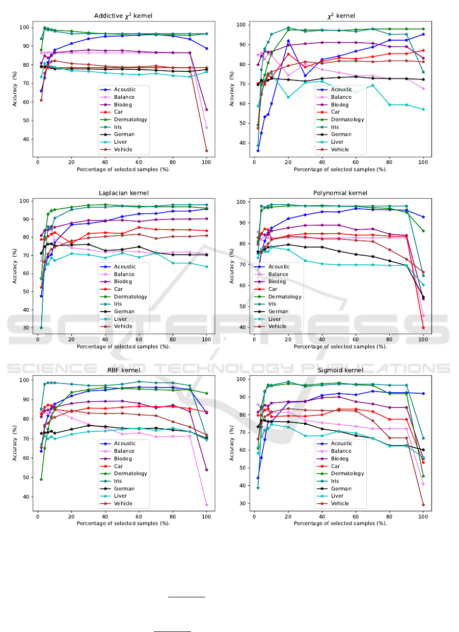
Figure 1: Accuracy (%) of training set pruning by genetic algorithm.
Experiments were conducted on 9 UCI datasets (see
Table 1 for an overview) using the following kernels:
• Addictive χ
2
kernel: k(x, y) = −
m
∑
i=1
(x
i
− y
i
)
2
x
i
+ y
i
• χ
2
kernel: k(x, y) = exp −γ
m
∑
i=1
(x
i
− y
i
)
2
x
i
+ y
i
!
• Laplacian kernel: k(x, y) = exp(−γ||x − y||)
• Polynomial kernel: k(x, y) = (γ < x, y > +c)
d
• RBF kernel: k(x, y) = exp(−γ||x − y||
2
)
• Sigmoid kernel: k(x, y) = tanh(γ < x, y > +c)
where x and y are two samples with m features, x
i
means the ith feature of sample x, and analog y
i
.
ICPRAM 2024 - 13th International Conference on Pattern Recognition Applications and Methods
432

Table 2: Accuracy (%) of training set pruning by genetic algorithm. For each dataset the optimal performance is marked bold.
Dataset
Reduction
2% 4% 6% 8% 10% 20% 30% 40% 50% 60% 70% 80% 90% 100%
Addictive χ
2
kernel
Acoustic 66.0 73.0 81.3 85.5 88.0 91.5 94.0 95.3 95.5 96.0 96.3 95.5 93.8 88.8
Balance 86.4 86.5 86.7 86.5 86.3 86.4 86.4 86.4 86.4 86.4 86.4 86.4 86.4 46.3
Biodeg 80.9 84.8 83.8 84.9 86.6 87.3 88.0 87.6 87.7 87.1 86.7 86.6 86.5 56.0
Car 78.9 78.5 78.5 78.5 78.5 78.5 78.5 78.5 78.5 78.5 78.5 78.5 78.5 78.5
Dermatology 88.0 100.0 99.4 98.9 98.6 98.1 97.2 96.7 96.4 96.7 96.1 96.1 95.8 96.7
Iris 94.0 99.3 98.7 98.7 98.0 96.7 96.7 96.7 96.7 96.7 96.7 96.7 96.7 96.7
German 79.2 79.2 79.2 78.5 77.8 77.8 77.8 77.6 77.7 77.5 77.1 76.6 76.5 77.5
Liver 73.6 80.9 79.4 79.1 78.8 76.8 76.5 75.7 75.1 74.8 75.4 74.2 73.6 76.2
Vehicle 61.0 75.5 79.8 81.8 82.2 80.7 80.2 79.3 78.8 78.9 79.5 78.4 78.6 33.9
χ
2
kernel
Acoustic 36.0 45.0 53.3 54.5 60.0 92.0 74.2 82.5 84.2 86.7 88.8 92.3 92.3 95.3
Balance 84.8 85.7 82.6 85.3 84.6 74.4 80.2 77.4 75.8 74.2 74.2 72.7 72.7 67.6
Biodeg 79.8 84.1 86.7 86.2 86.3 89.7 90.5 91.1 91.1 91.1 90.7 89.0 89.0 83.1
Car 70.3 71.0 69.7 74.4 73.3 85.2 78.6 81.5 83.3 82.8 83.9 85.4 85.4 87.1
Dermatology 49.2 69.6 74.6 80.8 85.5 97.5 97.5 97.5 97.2 97.7 98.0 98.0 98.0 98.0
Iris 38.7 77.3 88.0 91.3 95.3 98.7 96.7 97.3 97.3 96.7 98.0 95.3 95.3 76.0
German 69.6 71.9 70.9 71.9 72.8 72.2 71.4 72.8 73.3 73.7 72.9 72.7 72.7 72.3
Liver 58.8 65.5 71.9 75.4 75.1 63.2 70.7 71.3 67.5 65.8 69.3 59.4 59.4 57.1
Vehicle 47.5 64.7 71.2 75.0 76.2 79.3 81.3 80.5 81.7 81.7 81.3 81.8 81.8 81.3
Laplacian kernel
Acoustic 47.5 62.5 69.3 70.5 77.3 87.0 87.7 89 91.5 93.0 93.2 94.5 94.5 95.7
Balance 67.0 83.2 84.0 84.3 78.3 74.2 73.2 71.8 72.4 72.1 71.1 71.8 71.8 70.8
Biodeg 81.0 83.9 84.2 86.0 85.6 87.9 89.4 89.3 89.5 88.8 89.8 90.1 90.1 90.3
Car 78.9 78.8 80.6 81.8 82.7 76.7 82.1 82.6 82.1 85.5 84.4 84.2 84.2 83.7
Dermatology 57.1 80.3 92.8 94.7 95.3 96.7 97.8 98.1 97.5 97.2 96.9 96.9 96.9 96.1
Iris 30.0 66.7 86 84.7 90.7 95.3 96.7 96.7 97.3 96.7 97.3 98.0 98.0 98.0
German 71.2 74.8 76.3 76.4 75.4 75.8 76.1 72.7 73.3 74.8 71.5 70.4 70.4 70.3
Liver 57.7 63.8 65.2 68.7 67.2 71.0 70.4 68.7 71.3 69.0 71.3 65.8 65.8 63.8
Vehicle 52.4 66.4 70.8 73.4 74.6 78.1 79.7 80.5 81.1 81.7 79.4 80.5 80.5 81.0
Polynomial kernel
Acoustic 67.5 75.8 81.3 85.2 87.5 92.0 93.8 95.3 95.2 96.8 96.3 96.3 96.0 92.8
Balance 85.6 81.9 83.5 82.8 82.8 82.8 82.8 82.8 82.8 82.8 82.8 82.8 82.8 45.6
Biodeg 79.7 84.8 84.3 84.4 86.1 87.6 88.8 88.9 88.9 86.7 87.1 84.6 84.0 53.6
Car 82.9 84.8 87.1 86.7 82.1 83.9 84.8 84.8 84.9 84.1 84.2 83.6 83.6 39.8
Dermatology 81.0 95.8 97.2 97.2 97.5 98.1 98.1 98.3 98.0 97.8 97.2 96.9 95.0 86.1
Iris 75.3 98.0 97.3 98.0 98.7 98.7 98.0 98.0 98.0 98.0 98.0 98.0 98.0 64.7
German 76.2 76.3 77.2 78.4 78.5 79.6 78.4 78.4 76.4 74.9 73.9 71.8 69.6 54.5
Liver 73.3 77.4 76.2 76.2 78.3 77.1 71.9 70.4 69.9 69.9 69.9 69.6 69.6 60.3
Vehicle 63.7 76.1 78.4 80.0 81.9 83.5 83.2 82.2 82.3 81.6 81.1 77.1 72.6 66.4
RBF kernel
Acoustic 63.5 76.3 81.7 85.5 87.8 92.0 94.5 95.0 96.0 96.5 96.3 96.3 95.3 83.2
Balance 84.2 83.5 82.8 83.0 84.8 80.6 77.3 75.6 72.3 72.9 71.0 71.1 71.3 35.9
Biodeg 81.2 84.4 84.7 85.5 86.2 88.1 89.0 89.2 89.3 88.1 85.8 87.2 84.0 53.9
Car 82.7 86.1 87.3 87.0 85.0 83.9 85.7 85.5 86.1 86.6 86.4 86.4 85.5 83.7
Dermatology 49.0 65.1 74.9 81.3 84.9 93.8 95.2 96.3 95.8 95.5 95.2 94.9 95.2 93.3
Iris 85.3 98.0 98.7 98.7 98.7 98.0 97.3 97.3 98.0 99.3 98.7 98.7 97.3 70.7
German 72.7 73.0 73.2 73.8 72.8 74.8 76.7 76.2 75.3 75.1 75.4 74.4 73.6 70.1
Liver 67.0 71.3 69.9 71.0 69.9 72.2 73.6 73.9 74.8 75.4 74.2 75.4 73.6 69.3
Vehicle 65.4 76.9 77.9 80.4 81.0 84.4 83.1 82.9 83.0 82.3 81.8 78.7 76.0 71.9
Sigmoid kernel
Acoustic 44.3 55.8 66.0 76.3 76.0 80.7 87.5 91.0 92.0 91.3 93.3 92.5 92.5 92.0
Balance 85.8 83.0 82.7 82.5 81.1 81.5 76.9 75.5 74.5 73.5 72.1 72.1 72.1 40.8
Biodeg 81.5 83.9 85.4 84.9 86.6 87.4 87.6 89.6 90.1 87.4 86.1 84.1 84.1 55.2
Car 79.7 79.6 82.6 83.4 78.9 79.4 79.2 80.0 83.2 83.2 81.8 77.4 77.4 53.0
Dermatology 61.1 84.7 93.0 96.9 96.3 97.5 96.7 97.5 98.0 96.9 96.6 91.9 91.9 45.3
Iris 38.7 73.3 93.3 96.0 96.7 98.7 96.0 96.7 97.3 97.3 97.3 96.7 96.7 66.7
German 73.2 76.6 76.8 76.2 76.2 76.0 75.0 72.0 70.6 68.2 66.7 62.6 62.6 60.2
Liver 58.3 67.5 71.3 72.2 74.5 73.0 68.1 68.1 70.7 69.6 66.7 62.3 62.3 55.9
Vehicle 66.3 75.4 78.9 79.9 81.7 83.5 82.6 82.4 82.4 82.1 76.6 66.9 66.9 29.1
Classification Performance Boosting for Interpolation Kernel Machines by Training Set Pruning Using Genetic Algorithm
433

For the current study our intention is to demon-
strate the potential of training set pruning in general
and we did not optimize the parameters of the ker-
nels. Instead, we used the default settings of the used
software package. In our experiments we have used
Eq. (13) as fitness function.
We study different levels of pruning 2%, 4%, 6%,
8%, 10%, 20%, 30%, 40%, 50%, 60%, 70%, 80%,
90%. The use of the entire training set X is termed
as 100%. We conducted a 5-fold cross validation and
report the average performance in term of classifica-
tion accuracy. The experimental results are presented
in Figure 1 and Table 2 for details.
Generally, using the entire training set is not opti-
mal for classification performance. There are only a
few exceptions, e.g. dataset Acoustic with χ
2
kernel,
in our experiments. The optimal pruning level varies
dependent of the dataset and the used kernel. In many
cases even a reduction to ≤ 10% still maintains the
classification accuracy or is actually better. For the re-
duction level 10%, for instance, in 40 (74.1%) of the
54 test instances (9 datasets, 6 kernels) the classifica-
tion performance after training set pruning is identical
or even, partly significantly, superior to using the en-
tire training set. Even for the extreme reduction level
of 2% only, this ratio remains rather high (25 out of 54
test instances, 46.3%). In addition, there is typically
a broad range of pruning levels, where the classifi-
cation accuracy is superior to using the entire train-
ing set. A part of this broad range (approximately
between 20% and 80%) roughly shows a plateau of
high performance. Overall, our experimental results
confirmed the expected positive effect of training set
pruning on classification performance.
6 CONCLUSION
Recently, interpolation kernel machines have been
demonstrated to have several nice properties. In fact,
the study (Zhang et al., 2022) demonstrated that inter-
polation kernel machines are a good alternative to the
popular SVM. Motivated from different perspectives
of the curse of dimensionality we have studied train-
ing set pruning as a means of performance boosting
in this work. The experimental results clearly demon-
strated the potential for this purpose. In addition, the
significantly pruned training set also increases the ef-
ficiency in the test phase.
The current work shows the potential of training
set pruning only. We still need a mechanism to au-
tomatically determine the optimal reduction level in
order to really benefit from this potential in practice.
In addition, other metaheuristic optimization methods
such as particle swarm optimization can be applied
for training set pruning as well. We will study appli-
cations in specific domains, e.g. graphs. Interpola-
tion kernel machines can be a good choice for many
applications. With our work we contribute to increas-
ing the methodological plurality in machine learning
community.
ACKNOWLEDGEMENTS
Jiaqi Zhang was supported by the China Scholar-
ship Council (CSC). This research has received fund-
ing from the European Union’s Horizon 2020 re-
search and innovation programme under the Marie
Sklodowska-Curie grant agreement No 778602 Ultra-
cept.
REFERENCES
Angiulli, F. (2017). On the behavior of intrinsically high-
dimensional spaces: Distances, direct and reverse
nearest neighbors, and hubness. Journal of Machine
Learning Research, 18:170:1–170:60.
Belkin, M. (2021). Fit without fear: remarkable mathemat-
ical phenomena of deep learning through the prism of
interpolation. Acta Numerica, 30:203–248.
Belkin, M., Ma, S., and Mandal, S. (2018). To understand
deep learning we need to understand kernel learning.
In Proc. of 35th ICML, pages 540–548.
Birzhandi, P., Kim, K. T., and Youn, H. Y. (2022). Re-
duction of training data for support vector machine: a
survey. Soft Computing, 26(8):3729–3742.
Bishop, C. M. (2006). Pattern Recognition and Machine
Learning. Springer.
Burges, C. J. C. and Sch
¨
olkopf, B. (1996). Improving the
accuracy and speed of support vector machines. In
Advances in Neural Information Processing Systems
(NIPS), pages 375–381.
Chitnis, R. (2022). Refined lower bounds for nearest neigh-
bor condensation. In International Conference on Al-
gorithmic Learning Theory, pages 262–281.
Hady, M. F. A., Herbawi, W., Weber, M., and Schwenker, F.
(2011). A multi-objective genetic algorithm for prun-
ing support vector machines. In IEEE 23rd Interna-
tional Conference on Tools with Artificial Intelligence,
pages 269–275.
Han, M., Li, A., Gao, Z., Mu, D., and Liu, S. (2023). A
survey of multi-class imbalanced data classification
methods. Journal of Intelligent and Fuzzy Systems,
44(2):2471–2501.
Hang, H., Cai, Y., Yang, H., and Lin, Z. (2022). Under-
bagging nearest neighbors for imbalanced classifi-
cation. Journal of Machine Learning Research,
23:118:1–118:63.
ICPRAM 2024 - 13th International Conference on Pattern Recognition Applications and Methods
434

Heo, J., Lin, Z. L., and Yoon, S. (2019). Distance encoded
product quantization for approximate k-nearest neigh-
bor search in high-dimensional space. IEEE Trans.
PAMI, 41(9):2084–2097.
Herbrich, R. (2002). Learning Kernel Classifiers: Theory
and Algorithms. The MIT Press.
Houthuys, L. and Suykens, J. A. K. (2021). Tensor-based
restricted kernel machines for multi-view classifica-
tion. Information Fusion, 68:54–66.
Hsu, C. and Chen, M. (2009). On the design and applica-
bility of distance functions in high-dimensional data
space. IEEE Trans. Knowledge and Data Engineer-
ing, 21(4):523–536.
Huang, W., Du, W., and Xu, R. Y. D. (2021). On the neural
tangent kernel of deep networks with orthogonal ini-
tialization. In Proc. of 30th IJCAI, pages 2577–2583.
Hui, L., Ma, S., and Belkin, M. (2019). Kernel machines
beat deep neural networks on mask-based single-
channel speech enhancement. In Proc. of 20th INTER-
SPEECH, pages 2748–2752.
Jeong, Y., Hwang, M., and Sung, W. (2023). Training data
selection based on dataset distillation for rapid de-
ployment in machine-learning workflows. Multimedia
Tools and Applications, 82(7):9855–9870.
Kim, C. and Klabjan, D. (2020). A simple and fast algo-
rithm for L
1
-norm kernel PCA. IEEE Trans. PAMI,
42(8):1842–1855.
Lampert, C. H. (2009). Kernel methods in computer vision.
Foundations and Trends in Computer Graphics and
Vision, 4(3):193–285.
Ma, S. and Belkin, M. (2019). Kernel machines that adapt
to GPUs for effective large batch training. In Proc. of
3rd Conference on Machine Learning and Systems.
Motai, Y. (2015). Kernel association for classification and
prediction: A survey. IEEE Trans. Neural Networks
and Learning Systems, 26(2):208–223.
Nienk
¨
otter, A. and Jiang, X. (2023). Kernel-based gen-
eralized median computation for consensus learning.
IEEE Trans. PAMI, 45(5):5872–5888.
Nikolentzos, G., Siglidis, G., and Vazirgiannis, M. (2021).
Graph kernels: A survey. Journal of Artificial Intelli-
gence Research, 72:943–1027.
Nssibi, M., Manita, G., and Korbaa, O. (2023). Advances in
nature-inspired metaheuristic optimization for feature
selection problem: A comprehensive survey. Com-
puter Science Review, 49:100559.
Shanthi, D. L. and Chethan, N. (2023). Genetic algorithm
based hyper-parameter tuning to improve the perfor-
mance of machine learning models. SN Computer Sci-
ence, 4(2):119.
Shen, W., Lin, W., Wu, Y., Shi, F., Wu, W., and Li, K.
(2023). Evolving deep multiple kernel learning net-
works through genetic algorithms. IEEE Trans. In-
dustrial Informatics, 19(2):1569–1580.
Susan, S. and Kumar, A. (2019). SSO
maj
-SMOTE-
SSO
min
: Three-step intelligent pruning of majority
and minority samples for learning from imbalanced
datasets. Applied Soft Computing, 78:141–149.
Wang, R., Lu, J., Lu, Y., Nie, F., and Li, X. (2021). Discrete
multiple kernel k-means. In Proc. of 30th IJCAI, pages
3111–3117.
Wilson, D. R. and Martinez, T. R. (2000). Reduction tech-
niques for instance-based learning algorithms. Ma-
chine Learning, 38(3):257–286.
Winter, D., Bian, A., and Jiang, X. (2021). Layer-wise rele-
vance propagation based sample condensation for ker-
nel machines. In Proc. of 19th Int. Conf. on Computer
Analysis of Images and Patterns (CAIP), Part I, pages
487–496.
Wyner, A. J., Olson, M., Bleich, J., and Mease, D. (2017).
Explaining the success of AdaBoost and random
forests as interpolating classifiers. Journal of Machine
Learning Research, 18:48:1–48:33.
Xue, H. and Chen, S. (2014). Discriminality-driven reg-
ularization framework for indefinite kernel machine.
Neurocomputing, 133:209–221.
Yang, S., Xie, Z., Peng, H., Xu, M., Sun, M., and Li,
P. (2023). Dataset pruning: Reducing training data
by examining generalization influence. In 11th In-
ternational Conference on Learning Representations
(ICLR).
Zhang, J., Liu, C., and Jiang, X. (2022). Interpolation ker-
nel machine and indefinite kernel methods for graph
classification. In Proc. of 3rd Int. Conf. on Pattern
Recognition and Artificial Intelligence (ICPRAI), vol-
ume 13364 of LNCS, pages 467–479.
Classification Performance Boosting for Interpolation Kernel Machines by Training Set Pruning Using Genetic Algorithm
435