A Learning Paradigm for Interpretable Gradients
Felipe Torres Figueroa
1
, Hanwei Zhang
1
, Ronan Sicre
1
, Yannis Avrithis
2
and Stephane Ayache
1
1
Centrale Marseille, Aix Marseille Univ., CNRS, LIS, Marseille, France
2
Institute of Advanced Research on Artificial Intelligence (IARAI), Austria
Keywords:
Gradient, Guided Backpropagation, Class Activation Maps, Interpretability.
Abstract:
This paper studies interpretability of convolutional networks by means of saliency maps. Most approaches
based on Class Activation Maps (CAM) combine information from fully connected layers and gradient through
variants of backpropagation. However, it is well understood that gradients are noisy and alternatives like
guided backpropagation have been proposed to obtain better visualization at inference. In this work, we
present a novel training approach to improve the quality of gradients for interpretability. In particular, we
introduce a regularization loss such that the gradient with respect to the input image obtained by standard
backpropagation is similar to the gradient obtained by guided backpropagation. We find that the resulting gra-
dient is qualitatively less noisy and improves quantitatively the interpretability properties of different networks,
using several interpretability methods.
1 INTRODUCTION
The improvement of deep learning models in the last
decade has led to their adoption and penetration into
most application sectors. Since these models are
highly complex and opaque, the requirement for inter-
pretability of their predictions receives a lot of atten-
tion (Lipton, 2018). Explanation and transparency be-
comes a legal requirements for systems used in high-
stakes and high-risk decisions.
In this work, we focus on the visual interpretabil-
ity of deep learning models. Model interpretability
is often categorized into transparency and post-hoc
methods. Transparency aims at producing models
where the inner process or part of it can be under-
stood. Post-hoc methods consider models as black-
boxes and interpret decisions mainly based on inputs
and outputs.
In visual recognition, most methods focus on
post-hoc interpretability by means of saliency maps.
These maps highlight the most important areas of
an image related to the network prediction. Initial
works focused on using gradients for visualization,
such as guided backpropagation (Springenberg et al.,
2014). CAM (Zhou et al., 2016) later proposed a
class-specific linear combination of feature maps and
opened the way to numerous weighting strategies.
Most CAM-based methods use backpropagation
in one way or another. Recognizing that the gra-
dients obtained this way are noisy, methods like
SmoothGrad (Smilkov et al., 2017) and SmoothGrad-
CAM++ (Omeiza et al., 2019) improve the quality of
saliency maps by denoising the gradients. However,
this requires several forward passes, thus comes with
increased cost at inference.
In this work, we rather propose a learning
paradigm for model training that regularizes gradients
to improve the performance of interpretability meth-
ods. In particular, we add a regularization term to the
loss function that encourages the gradient in the input
space to align with the gradient obtained by guided
back-propagation. This has a smoothing effect on gra-
dient and is shown to improve the power of model in-
terpretations.
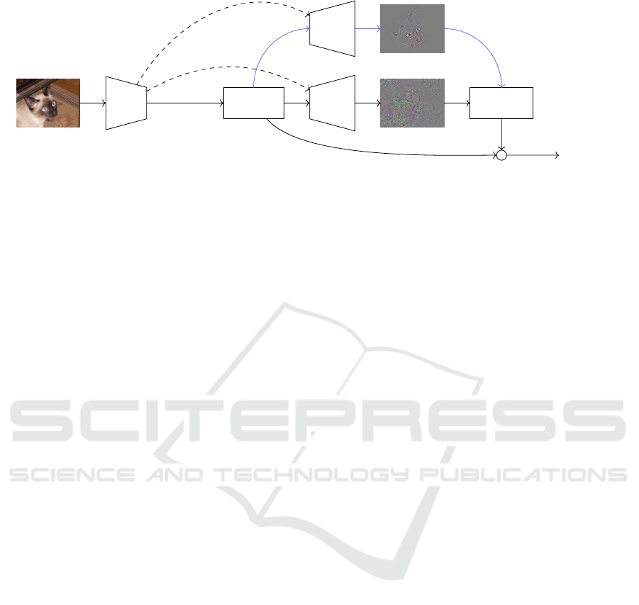
Figure 1 summarizes our method. At training,
each input image is forwarded through the network to
compute the cross-entropy loss. Standard and guided
backpropagation is performed back to the input im-
age space, where our regularization term is computed.
This term is added to the loss and backpropagated
only through the standard backpropagation branch.
The key contributions of this work are as follows:
• We introduce a new learning paradigm to regular-
ize gradients.
• Using different networks, we show that our
method improves the gradient quality and the per-
formance of several interpretability methods us-
ing multiple metrics, while preserving accuracy.
Figueroa, F., Zhang, H., Sicre, R., Avrithis, Y. and Ayache, S.
A Learning Paradigm for Interpretable Gradients.
DOI: 10.5220/0012466800003660
Paper published under CC license (CC BY-NC-ND 4.0)
In Proceedings of the 19th International Joint Conference on Computer Vision, Imaging and Computer Graphics Theory and Applications (VISIGRAPP 2024) - Volume 3: VISAPP, pages
757-764
ISBN: 978-989-758-679-8; ISSN: 2184-4321
Proceedings Copyright © 2024 by SCITEPRESS – Science and Technology Publications, Lda.
757

guided
backprop
∂
G
L
C
/∂x
input image x
network
f
classification
loss L
C
standard
backprop
∂L
C
/∂x
regularization
loss L
R
+
total loss
L = L
C
+ λL
R
logits y
//
stop gradient
Figure 1: Interpretable gradient learning. For an input image x, we obtain the logit vector y = f (x; θ ) by a forward pass
through the network f with parameters θ. We compute the classification loss L
C
by softmax and cross-entropy (6), (7).
We obtain the standard gradient ∂L
C
/∂x and guided gradient ∂
G
L
C
/∂x by two backward passes (dashed) and compute the
regularization loss L
R
as the error between the two (8),(10)-(12). The total loss is L = L
C
+ λL
R
(9). Learning is based on
∂L/∂θ, which involves differentiation of the entire computational graph except the guided backpropagation branch (blue).
2 RELATED WORK
Interpretability of deep neural network decisions is
a problem that receives increasing interest. As in-
terpretability is not simple to define, Lipton (Lipton,
2018) proposes some common ground, definitions
and categorization for interpretability methods. For
instance, transparency aims at making models simple
so it is humanly possible to provide an explanation of
its inner mechanism. By contrast, post-hoc methods
consider models as black boxes and study the activa-
tions leading to a specific output.
LIME (Ribeiro et al., 2016) and SHAP (Lundberg
and Lee, 2017) are probably the most popular post-
hoc methods that are model agnostic and provide lo-
cal information. Concerning image recognition tasks,
it is common to generate saliency maps highlighting
the areas of an image that are responsible for a spe-
cific prediction. Several of these methods are either
based on backpropagation and its variants or on Class
Activation Maps (CAM) that weigh the importance of
activation maps.
2.1 Gradient-Based Approaches
Gradient-based approaches assess the impact of dis-
tinct image regions on the prediction based on the par-
tial derivative of the model prediction function with
respect to the input. A simple saliency map can be
the partial derivative obtained by a single backward
pass through the model (Simonyan et al., 2014).
Guided backpropagation (Springenberg et al.,
2014) enhances explanations by removing negative
gradients through ReLU units. For better visualiza-
tion, SmoothGrad (Smilkov et al., 2017) applies noise
to the input and derives saliency maps based on the
average of resulting gradients. Layer-wise Relevance
Propagation (LRP) (Bach et al., 2015) reallocates
the prediction score through a custom backward pass
across the network.
Our method has a similar objective as Smooth-
Grad (Smilkov et al., 2017) but instead of using sev-
eral forward passes at inference, we regularize gra-
dients using guided backpropagation during training.
Thus we obtain better gradients without modifying
the inference process and our method can be used
with any interpretability method at inference.
2.2 CAM-Based Approaches
Class Activation Maps (Zhou et al., 2016) produces
a saliency map that highlights the areas of an image
that are the most responsible for a CNN decision. The
saliency map is computed as a linear combinations of
feature maps from a given layer. Different variants
of CAM are proposed by defining different weighting
coefficients. Grad-CAM (Selvaraju et al., 2017), for
instance, spatially averages the gradient with respect
to feature maps. Grad-CAM++ (Chattopadhay et al.,
2018) improves object localization by using positive
partial derivatives and measuring recognition and lo-
calization metrics.
It is possible to extend CAM to multiple lay-
ers (Jiang et al., 2021) and to improve sensi-
tivity (Sundararajan et al., 2017) and conserva-
tion (Montavon et al., 2018) by the addition of ax-
ioms (Fu et al., 2020). Score-CAM (Wang et al.,
2020) is a gradient-free method that computes weight-
ing coefficients by maximizing the Average Increase
metric (Chattopadhay et al., 2018). Further improve-
VISAPP 2024 - 19th International Conference on Computer Vision Theory and Applications
758

ment can be obtained by means of test-time optimiza-
tion (Zhang et al., 2023).
Some works provide explanations that not only lo-
calize salient parts of images, but also provide theo-
retical bases on the effect of modifying such regions
for a given input (Fu et al., 2020). An exhaustive al-
ternative performs ablation experiments to highlight
such parts (Ramaswamy et al., 2020).
All these approaches apply at inference, without
modifying the model or the training process. By con-
trast, our work applies at training with the objec-
tive of improving the quality of gradients, which is
much needed for gradient-based methods. Thus, our
method is orthogonal and can be used with any of
these approaches at inference.
2.3 Double Backpropagation
Double backpropagation is a general regulariza-
tion paradigm, first introduced by Drucker and Le
Cun (Drucker and Le Cun, 1991) to improve general-
ization. The idea is used to avoid overfitting (Philipp
and Carbonell, 2018), help transfer (Srinivas and
Fleuret, 2018), cope with noisy labels (Luo et al.,
2019), and more recently to increase adversarial ro-
bustness (Lyu et al., 2015; Simon-Gabriel et al., 2018;
Ross and Doshi-Velez, 2018; Seck et al., 2019; Finlay
et al., 2018). It aims at penalizing the 
1
(Seck et al.,
2019), 
2
or 
∞
norm of the gradient with respect to
the input image.
Our method is related and regularizes the stan-
dard gradient by aligning it with the guided gradi-
ent, obtained by guided backpropagation (Springen-
berg et al., 2014).
3 BACKGROUND
3.1 Guided Backpropagation
The derivative of v = ReLU(u) = [u]
+
= max(u,0)
with respect to u is dv/du =
u>0
. By the chain rule,
a signal δv = ∂L/∂v is then propagated backwards
through the ReLU unit to δu = ∂L/∂u as δu =
u>0
δv,
where ∂L/∂v is the partial derivative of any scalar
quantity of interest, e.g. a loss L, with respect to v.
Guided backpropagation (Springenberg et al.,
2014) changes this to δ
G
u =
u>0
[δv]
+
, masking out
values corresponding to negative entries of both the
forward (u) and the backward (δv) signals and thus
preventing backward flow of negative gradients.
Standard backpropagation through an entire net-
work f with this particular change for ReLU units
is called guided backpropagation. The correspond-
ing guided “partial derivative” or guided gradient of
scalar quantity L with respect to v is denoted by
∂
G
L/∂v. This method allows sharp visualization of
high-level activations conditioned on input images.
3.2 CAM-Based Methods
CAM-based methods build a saliency map as a linear
combination of feature maps. Given a target class c
and a set of 2D feature maps {A
k
}
K
k=1
, the saliency
map is defined as
S
c
= ReLU
K
∑
k=1
α
c
k
A
k
!
, (1)
where the weight α
c
k
determines the contribution of
channel k to class c. The saliency map S
c
and the
feature maps A
k
are both non-negative because of
using ReLU activation functions. Different CAM-
based methods differ primarily in the definition of the
weights α
c
k
.
CAM (Zhou et al., 2016) originally defines α
c
k
as
the weight connecting channel k to class c in the clas-
sifier, assuming {A
k
} are the feature maps of the last
convolutional layer, which is followed by global av-
erage pooling (GAP) and a fully connected layer.
Grad-CAM (Selvaraju et al., 2017) is a general-
ization of CAM for any network. If y
c
is the logit of
class c, the weights are obtained by GAP of the partial
derivatives of y
c
with respect to elements of feature
map A
k
of any given layer,
α
c
k
=
1
Z
∑
i, j
∂y
c
∂A
k
i j
, (2)
where A
k
i j
denotes the value at spatial location (i, j) of
feature map A
k
and Z is the total number of locations.
Guided Grad-CAM elementwise-multiplies the
saliency maps obtained by Grad-CAM and guided
backpropagation, after adjusting spatial resolu-
tions. The resulting visualizations are both class-
discriminative (by Grad-CAM) and contain fine-
grained detail (by guided backpropagation).
Grad-CAM++ (Chattopadhay et al., 2018) is a
generalization of Grad-CAM, where partial deriva-
tives of y
c
with respect to A
k
are followed by ReLU as
in guided backpropagation and GAP is replaced by a
weighted average:
a
c
k
=
∑
i, j
w
kc
i j
ReLU
∂y
c
∂A
k
i j
!
. (3)
A Learning Paradigm for Interpretable Gradients
759

The weights w
kc
i j
of the linear combination are
w
kc
i j
=
∂
2
y
c
∂(A
k
i j
)
2
2
∂
2
y
c
∂(A
k
i j
)
2
+
∑
a,b
A
k
ab
∂
3
y
c
∂(A
k
i j
)
3
. (4)
Score-CAM (Wang et al., 2020) computes the
weights a
c
k
based on the increase in confidence (Chat-
topadhay et al., 2018) for class c obtained by mask-
ing (element-wise multiplying) the input image x with
feature map A
k
:
a
c
k
= f (x ◦ s(Up(A
k
)))
c
− f (x
b
)
c
, (5)
where Up is upsampling to the spatial resolution of
x, s is linear normalization to range [0,1], ◦ is the
Hadamard product, f is the network mapping of input
image to class probability vectors and x
b
is a baseline
image.
While Score-CAM does not require gradients to
compute saliency maps, (5) requires one forward pass
through the network f for each channel k.
4 METHOD
Preliminaries. We consider an image classification
network f with parameters θ, which maps an input
image x to a vector of predicted class probabilities
p = f (x; θ). At inference, we predict the class of max-
imum confidence argmax
j
p
j
, where p
j
is the proba-
bility of class j. At training, given training images
X = {x
i
}
n
i=1
and target labels T = {t
i
}
n
i=1
, we com-
pute the classification loss
L
C
(X,θ,T ) =
1
n
n
∑
i=1
CE( f (x
i
;θ),t
i
), (6)
where CE is cross-entropy:
CE(p,t) = −log p
t
. (7)
Updates of parameters θ are performed by an opti-
mizer, based on the standard partial derivative (gradi-
ent) ∂L
C
/∂θ of the classification loss L
C
with respect
to θ, obtained by standard back-propagation.
Motivation. Due to non-linearities like ReLU acti-
vations and downsampling like max-pooling or con-
volution stride greater than 1, the standard gradient is
noisy (Smilkov et al., 2017). This is shown by visu-
alizing the gradient ∂L
C
/∂x with respect to an input
image x. By contrast, the guided gradient ∂
G
L
C
/∂x
(Springenberg et al., 2014) does not suffer much from
noise and preserves sharp details. The difference of
the two gradients is illustrated in Figure 1.
The main motivation of this work is that introduc-
ing a regularization term during training could make
the standard gradient ∂L
C
/∂x behave similarly to the
corresponding guided gradient ∂
G
L
C
/∂x, while main-
taining the predictive power of the classifier f . We hy-
pothesize that, if this is possible, it will improve the
quality of all gradients with respect to intermediate
activations and therefore the quality of saliency maps
obtained by CAM-based methods (Zhou et al., 2016;
Selvaraju et al., 2017; Chattopadhay et al., 2018;
Wang et al., 2020) and the interpretability of network
f . The effect may be similar to that of SmoothGrad
(Smilkov et al., 2017), but without the need for sev-
eral forward passes at inference.
Regularization. Given an input training image x
i
and its target labels t
i
, we perform a forward pass
through f and compute the probability vectors p
i
=
f (x
i
,θ) and the contribution of (x
i
,t
i
) to the classifi-
cation loss L
C
(X,θ,T ) (6).
We then obtain the standard gradients δx
i
=
∂L
C
/∂x
i
and the guided gradients δ
G
x
i
= ∂
G
L
C
/∂x
i
with respect to x
i
by two separate backward passes.
Since the whole process is differentiable (w.r.t. θ) at
training, we stop the gradient computation of the lat-
ter, so that it only serves as a “teacher”. We define the
regularization loss
L
R
(X,θ,T ) =
1
n
n
∑
i=1
E(δx
i
,δ
G
x
i
), (8)
where E is an error function between the two gradient
images, considered below.
The total loss is defined as
L(X,θ,T ) = L
C
(X,θ,T ) + λL
R
(X,θ,T ), (9)
where λ is a hyperparameter determining the regular-
ization strength. λ should be large enough to smooth
the gradient without decreasing the classification ac-
curacy or harming the training process.
Updates of the network parameters θ are based on
the standard gradient ∂L/∂θ of the total loss L w.r.t.
θ, using any optimizer. At inference, one may use
any interpretability method to obtain a saliency map
at any layer.
Error Function. Given two gradient images δ,δ
0
consisting of m pixels each, we consider the follow-
ing error functions E to compute the regularization
loss (8).
1. Mean absolute error (MAE):
E
MAE
(δ,δ
0
) =
1
m


δ − δ
0


1
. (10)
2. Mean squared error (MSE):
E
MSE
(δ,δ
0
) =
1
m


δ − δ
0


2
2
. (11)
We also consider the following two similarity
functions, with a negative sign.
VISAPP 2024 - 19th International Conference on Computer Vision Theory and Applications
760

3. Cosine similarity:
E
cos
(δ,δ
0
) = −
h
δ,δ
0
i
k
δ
k
2
k
δ
0
k
2
, (12)
where
h
,
i
denotes inner product.
4. Histogram intersection (HI):
E
HI
(δ,δ
0
) = −
∑
m
i=0
min(
|
δ
i
|
,
|
δ
0
i
|
)
k
δ
k
1
k
δ
0
k
1
. (13)
Algorithm. Our method is summarized in algo-
rithm 1 and illustrated in Figure 1. It is interest-
ing to note that the entire computational graph de-
picted in Figure 1 involves one forward and two back-
ward passes. This graph is then differentiated again
to compute ∂L/∂θ, which involves one more forward
and backward pass, since the guided backpropagation
branch is excluded. Thus, each training iteration re-
quires five passes through f instead of two in standard
training.
Algorithm 1: Interpretable gradient loss.
Input: network f , parameters θ
Input: input images X = {x
i
}
n
i=1
Input: target labels T = {t
i
}
n
i=1
Output: loss L
L
C
←
1
n
∑
n
i=1
CE( f (x
i
;θ),t
i
)  class. loss (6)
foreach i ∈ {1,... ,n} do
δx
i
← ∂L
C
/∂x
i
 standard grad
δ
G
x
i
← ∂
G
L
C
/∂x
i
 guided grad
DETACH(δ
G
x
i
)  detach from graph
L
R
←
1
n
∑
n
i=1
E(δx
i
,δ
G
x
i
)  reg. loss (8)
L ← L
C
+ λL
R
 total loss (9)
5 EXPERIMENTS
5.1 Experimental Setup
In the following sections, we evaluate the effect of our
approach on recognition and interpretability.
Models and Datasets. We train and evaluate a
ResNet-18 (He et al., 2016) and a MobileNet-
V2 (Sandler et al., 2018) on CIFAR-100 (Krizhevsky,
2009). ResNets are the most common CNNs and
the ResNet-18 is particularly adapted to low resolu-
tion images. MobileNet-V2 is a widely used com-
pact CNN. CIFAR-100 contains 60.000 images of 100
categories, split in 50.000 for training and 10.000 for
testing. Each image has a resolution of 32×32 pixels.
Settings. To obtain competitive performance and
ensure the replicability of our method, we follow the
methodology by weiaicunzai
1
. In particular, we train
for 200 epochs, with a batch-size of 128 images, SGD
optimizer, initial learning rate 10
−1
and learning rate
decay by a factor of 5 on epochs 60, 120 and 160.
At inference, we generate explanations fol-
lowing popular attribution methods derived from
CAM (Zhou et al., 2016), from the pytorch-grad-cam
library from Jacob Gildenblat
2
.
5.2 Faithfulness Metrics
Faithfulness evaluation (Chattopadhay et al., 2018)
offers insight on the regions of an image that are con-
sidered important for recognition, as highlighted by
the saliency map S
c
. Specifically, given a target class
c, an image x and a saliency map S
c
are element-wise
multiplied to obtain a masked image
m
c
= S
c
◦ x.
This masked image is similar to the original image
on the salient areas and black on the non-salient ones.
To evaluate the quality of saliency maps, we forward
both the original image x and its masked version m
c
through the network to obtain the predicted probabil-
ities p
c
i
and o
c
i
respectively. We then compute a num-
ber of metrics as defined below.
Average Drop (AD). aims at quantifying how much
predictive power is lost when we consider the masked
image compared to the original one. Lower is better.
AD =
1
N
N
∑
i=1
[p
c
i
− o
c
i
]
+
p
c
i
. (14)
Average Increase (AI). is also known as Increase
of Confidence and measures the percentage of exam-
ples of the dataset where the masked image offers
a higher probability than the original for the target
class. Higher is better.
AI =
1
N
N
∑
i
(p
c
i
< o
c
i
). (15)
Average Gain (AG). is recently introduced
in (Zhang et al., 2023) and designed to be a sym-
metric complement of AD, replacing AI. It aims at
quantifying how much predictive power is gained
when we consider the masked image compared to the
original one. Higher is better.
AG =
1
N
N
∑
i=1
[o
c
i
− p
c
i
]
+
p
c
i
. (16)
1
https://github.com/weiaicunzai/pytorch-cifar100
2
https://github.com/jacobgil/pytorch-grad-cam
A Learning Paradigm for Interpretable Gradients
761

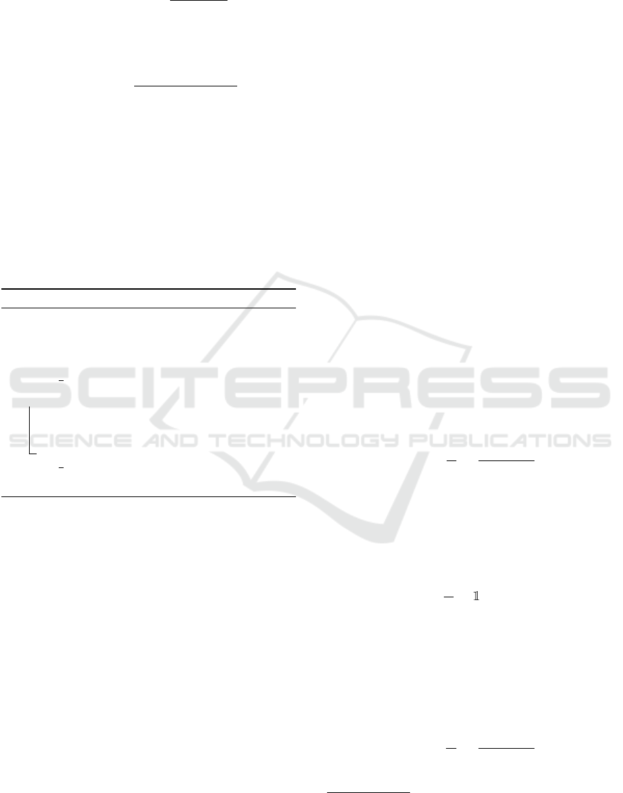
INPUT
GRAD-CAM GRAD-CAM++ SCORE-CAM ABLATION-CAM
BASELINE OURS BASELINE OURS BASELINE OURS BASELINE OURS
Man
Girl
Woman
Lobster
Couch
Figure 2: Saliency map comparison of standard vs. our training using different CAM-based methods on CIFAR-100 examples.
5.3 Causal Metrics
Causality evaluation (Petsiuk et al., 2018) aims at
evaluating the effect of masking certain elements of
the image in the predictive power of a model. Two
metrics are defined as follows. Histograms and av-
erage values can be computed per image. Follow-
ing most previous work, we only show average values
over the test set.
Insertion. starts from a blurry image and gradually
inserts (unblurs) pixels of the original image, ranked
by decreasing saliency as defined in a given saliency
map. At each iteration, images are passed through the
network to compute the predicted probabilities and
compare to the original.
Deletion. gradually removes the pixels by replacing
them by black, starting from the most salient pixels.
As for insertion, we compute the predicted probabili-
ties at each iteration.
5.4 Qualitative Results
We visualize the effect of our approach on saliency
maps and gradients, obtained for the baseline model
vs. the one trained with our approach.
Figure 2 shows saliency maps. We observe the
differences brought by our training method. The dif-
ferences are particularly important for Grad-CAM,
which directly averages the gradient to weigh feature
maps. Interestingly, the differences are smaller for
Score-CAM, which is not gradient-based but only ob-
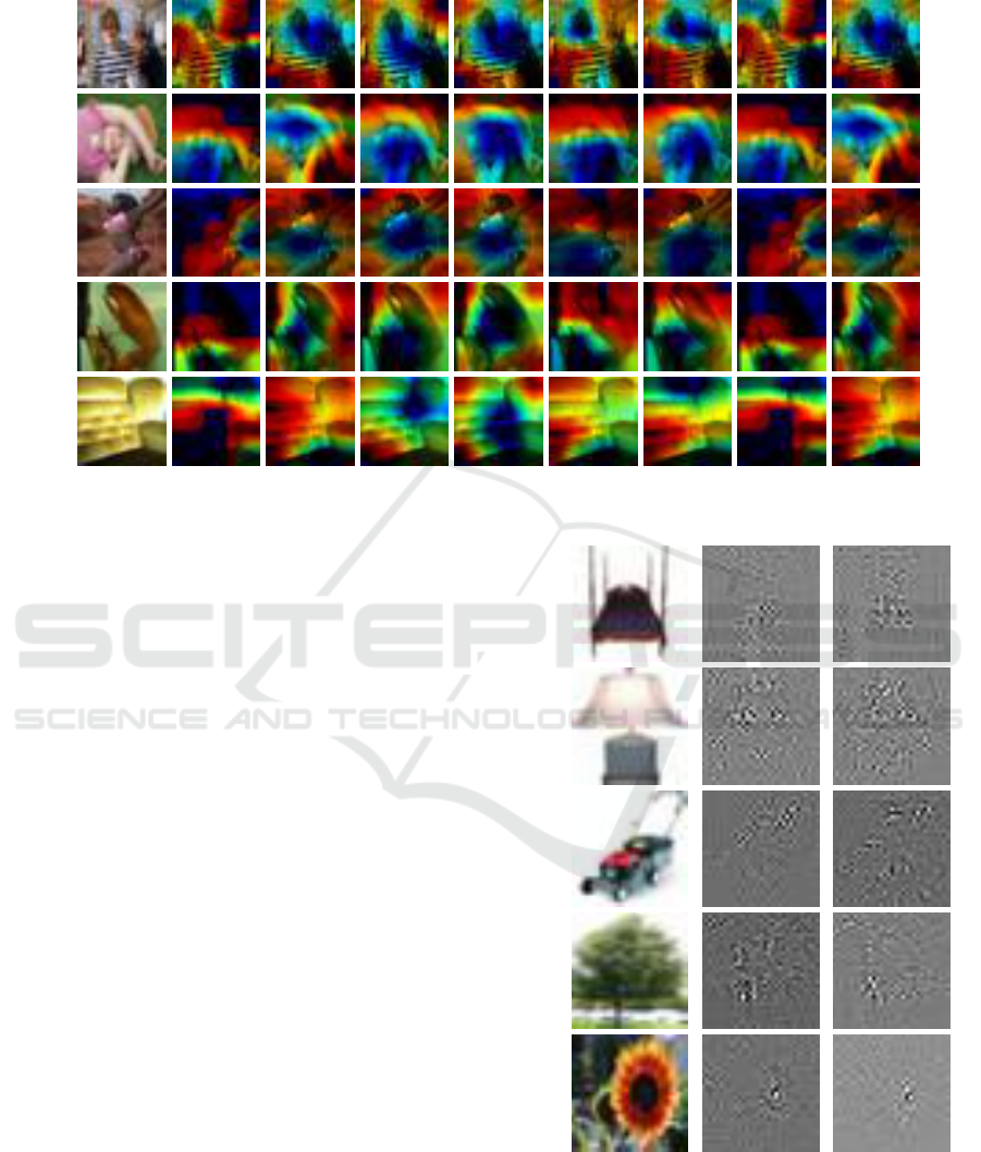
INPUT BASELINE OURS
Bed
Lamp
Lawnmower
Maple Tree
Sunflower
Figure 3: Gradient comparison of standard vs. our training
on CIFAR-100 examples.
tains changes of predicted probabilities.
Figure 3 shows gradients. We observe slightly less
noise with our method, while the object of interest is
VISAPP 2024 - 19th International Conference on Computer Vision Theory and Applications
762

Table 1: Accuracy of standard vs. our training using
ResNet-18 and MobileNet-V2 on CIFAR-100. Using co-
sine error function for our training.
MODEL ERROR λ ACC
RESNET-18
Baseline – 73.42
Ours 7.5 × 10
−3
72.86
MOBILENET-V2
Baseline – 59.43
Ours 1 × 10
−3
62.36
Table 2: Interpretability metrics of standard vs. our training
using ResNet-18 and MobileNet-V2 on CIFAR-100. Using
cosine error function for our training.
RESNET-18
METHOD ERROR AD↓ AG↑ AI↑ INS↑ DEL↓
GRAD-CAM
Baseline 30.16 15.23 29.99 58.47 17.47
Ours 28.09 16.19 31.53 58.76 17.57
GRAD-CAM++
Baseline 31.40 14.17 28.47 58.61 17.05
Ours 29.78 15.07 29.60 58.90 17.22
SCORE-CAM
Baseline 26.49 18.62 33.84 58.42 18.31
Ours 24.82 19.49 35.51 59.11 18.34
ABLATION-CAM
Baseline 31.96 14.02 28.33 58.36 17.14
Ours 29.90 15.03 29.61 58.70 17.37
AXIOM-CAM
Baseline 30.16 15.23 29.98 58.47 17.47
Ours 28.09 16.20 31.53 58.76 17.57
MOBILENET-V2
METHOD ERROR AD↓ AG↑ AI↑ INS↑ DEL↓
GRAD-CAM
Baseline 44.64 6.57 25.62 44.64 14.34
Ours 40.89 7.31 27.08 45.57 15.20
GRAD-CAM++
Baseline 45.98 6.12 24.10 44.72 14.76
Ours 40.76 6.85 26.46 45.51 14.92
SCORE-CAM
Baseline 40.55 7.85 28.57 45.62 14.52
Ours 36.34 9.09 30.50 46.35 14.72
ABLATION-CAM
Baseline 45.15 6.38 25.32 44.62 15.03
Ours 41.13 7.03 26.10 45.38 15.12
AXIOM-CAM
Baseline 44.65 6.57 25.62 44.64 15.27
Ours 40.89 7.31 27.08 45.57 15.20
better covered by gradient activations.
5.5 Quantitative Results
We evaluate the effect of training a given model using
our proposed approach with faithfulness and causal-
ity metrics. As shown in Table 1 and Table 2, we
obtain improvements on both networks and on four
out of five interpretability metrics, while remaining
within half percent or improving accuracy relative to
the baseline, standard backpropagation.
The improvements are higher for faithfulness met-
rics AD, AG, and AI. Insertion gets a smaller but con-
sistent improvement. Deletion is mostly inferior with
our method, but with a very small difference. This
may be due to limitations of the metrics, as reported
in previous works (Zhang et al., 2023).
Table 3: Effect of error function on our approach, using
ResNet-18 and Grad-CAM attributions on CIFAR-100.
ERROR FUNCTION ACC AD↓ AG↑ AI↑ INS↑ DEL↓
Baseline 73.42 30.16 15.23 29.99 58.47 17.47
Cosine 72.86 28.09 16.19 31.53 58.76 17.57
Histogram 73.88 30.39 14.78 29.38 58.52 17.35
MAE 73.41 30.33 15.06 29.61 58.13 17.95
MSE 73.86 29.64 15.19 30.11 59.05 18.02
Table 4: Effect of regularization coefficient λ (9) on our
approach, using ResNet-18 and Grad-CAM attributions on
CIFAR-100. Using cosine error function for our training.
λ ACC AD↓ AG↑ AI↑ INS↑ DEL↓
0 73.42 30.16 15.23 29.99 58.47 17.47
1 × 10
−3
73.71 29.52 15.17 30.03 59.23 17.45
2.5 × 10
−3
72.99 30.53 15.82 30.56 59.04 17.96
5 × 10
−3
72.46 30.10 16.06 30.67 57.47 17.80
7.5 × 10
−3
72.86 28.09 16.20 31.53 58.76 17.57
1 × 10
−2
73.28 28.97 15.75 31.16 58.99 17.50
1 × 10
−1
73.00 28.93 16.13 31.55 59.66 17.95
1 73.30 28.44 16.02 31.31 58.64 17.48
10 73.04 29.28 15.23 30.47 58.74 17.47
It is interesting to note that improvements on
Score-CAM mean that our training not only improves
gradient but also builds better activation maps, since
Score-CAM only relies on those.
5.6 Ablation Experiments
Using ResNet-18 and Grad-CAM attributions, we an-
alyze the effect of the error function and the regular-
ization coefficient λ (9) on our approach.
Error Function. As shown in Table 3, we obtain a
consistent improvement on most metrics for all error
functions. Accuracy remains stable within half per-
cent of the original model. However, most options
have little or negative effect on deletion. Cosine sim-
ilarity provides improvements in most metrics, while
maintaining deletion performance. We thus choose
cosine error function by default.
Regularization Coefficient. As shown in Table 4,
our method is not very sensible to the regularization
coefficient λ. The value of 7.5 ×10
−3
works better in
general and is thus selected as default.
6 CONCLUSION
In this paper, we propose a new training approach
to improve the gradient of a CNN in terms of inter-
pretability. Our method forces the gradient with re-
A Learning Paradigm for Interpretable Gradients
763

spect to the input image obtained by backpropaga-
tion to align with the gradient coming from guided
backpropagation. The results of our training are eval-
uated according to several interpretability methods
and metrics. Our method offers consistent improve-
ment on most metrics for two networks, while remain-
ing within a small margin of the standard gradient in
terms accuracy.
REFERENCES
Bach, S., Binder, A., Montavon, G., Klauschen, F., M
¨
uller,
K.-R., and Samek, W. (2015). On pixel-wise explana-
tions for non-linear classifier decisions by layer-wise
relevance propagation. PloS one, 10(7).
Chattopadhay, A., Sarkar, A., Howlader, P., and Balasub-
ramanian, V. N. (2018). Grad-CAM++: Generalized
gradient-based visual explanations for deep convolu-
tional networks. In WACV.
Drucker, H. and Le Cun, Y. (1991). Double backpropaga-
tion increasing generalization performance. In IJCNN.
Finlay, C., Oberman, A. M., and Abbasi, B. (2018). Im-
proved robustness to adversarial examples using Lip-
schitz regularization of the loss.
Fu, R., Hu, Q., Dong, X., Guo, Y., Gao, Y., and Li, B.
(2020). Axiom-based Grad-CAM: Towards accurate
visualization and explanation of CNNs. arXiv preprint
arXiv:2008.02312.
He, K., Zhang, X., Ren, S., and Sun, J. (2016). Deep resid-
ual learning for image recognition. In CVPR.
Jiang, P.-T., Zhang, C.-B., Hou, Q., Cheng, M.-M., and Wei,
Y. (2021). LayerCAM: Exploring hierarchical class
activation maps for localization. TIP.
Krizhevsky, A. (2009). Learning multiple layers of features
from tiny images. pages 32–33.
Lipton, Z. C. (2018). The mythos of model interpretability:
In machine learning, the concept of interpretability is
both important and slippery. Queue, 16(3):31–57.
Lundberg, S. M. and Lee, S.-I. (2017). A unified approach
to interpreting model predictions. In NeurIPS.
Luo, Y., Zhu, J., and Pfister, T. (2019). A simple yet ef-
fective baseline for robust deep learning with noisy
labels. arXiv preprint arXiv:1909.09338.
Lyu, C., Huang, K., and Liang, H.-N. (2015). A unified gra-
dient regularization family for adversarial examples.
In international conference on data mining.
Montavon, G., Samek, W., and M
¨
uller, K.-R. (2018). Meth-
ods for interpreting and understanding deep neural
networks. Digital Signal Processing, 73:1–15.
Omeiza, D., Speakman, S., Cintas, C., and Weldermariam,
K. (2019). Smooth Grad-CAM++: An enhanced in-
ference level visualization technique for deep con-
volutional neural network models. arXiv preprint
arXiv:1908.01224.
Petsiuk, V., Das, A., and Saenko, K. (2018). RISE: Ran-
domized input sampling for explanation of black-box
models. arXiv preprint arXiv:1806.07421.
Philipp, G. and Carbonell, J. G. (2018). The nonlinear-
ity coefficient-predicting generalization in deep neural
networks. arXiv preprint arXiv:1806.00179.
Ramaswamy, H. G. et al. (2020). Ablation-CAM: Vi-
sual explanations for deep convolutional network via
gradient-free localization. In WACV.
Ribeiro, M. T., Singh, S., and Guestrin, C. (2016). ” why
Should I Trust You?” explaining the Predictions of
Any Classifier. In SIGKDD.
Ross, A. S. and Doshi-Velez, F. (2018). Improving the ad-
versarial robustness and interpretability of deep neu-
ral networks by regularizing their input gradients. In
AAAI.
Sandler, M., Howard, A., Zhu, M., Zhmoginov, A., and
Chen, L.-C. (2018). MobileNetv2: Inverted residuals
and linear bottlenecks. In CVPR.
Seck, I., Loosli, G., and Canu, S. (2019). L 1-norm double
backpropagation adversarial defense. arXiv preprint
arXiv:1903.01715.
Selvaraju, R. R., Cogswell, M., Das, A., Vedantam, R.,
Parikh, D., and Batra, D. (2017). Grad-CAM: Visual
explanations from deep networks via gradient-based
localization. In ICCV.
Simon-Gabriel, C.-J., Ollivier, Y., Bottou, L., Sch
¨
olkopf,
B., and Lopez-Paz, D. (2018). Adversarial vulnerabil-
ity of neural networks increases with input dimension.
Simonyan, K., Vedaldi, A., and Zisserman, A. (2014).
Deep inside convolutional networks: Visualising im-
age classification models and saliency maps. ICLR
Workshop.
Smilkov, D., Thorat, N., Kim, B., Vi
´
egas, F., and Watten-
berg, M. (2017). Smoothgrad: removing noise by
adding noise. arXiv preprint arXiv:1706.03825.
Springenberg, J. T., Dosovitskiy, A., Brox, T., and Ried-
miller, M. (2014). Striving for simplicity: The all con-
volutional net. arXiv preprint arXiv:1412.6806.
Srinivas, S. and Fleuret, F. (2018). Knowledge transfer with
jacobian matching. In International Conference on
Machine Learning, pages 4723–4731. PMLR.
Sundararajan, M., Taly, A., and Yan, Q. (2017). Axiomatic
attribution for deep networks. In ICML.
Wang, H., Wang, Z., Du, M., Yang, F., Zhang, Z., Ding, S.,
Mardziel, P., and Hu, X. (2020). Score-CAM: Score-
weighted visual explanations for convolutional neural
networks. In CVPR work.
Zhang, H., Torres, F., Sicre, R., Avrithis, Y., and Ayache,
S. (2023). Opti-CAM: Optimizing saliency maps for
interpretability. arXiv preprint arXiv:2301.07002.
Zhou, B., Khosla, A., Lapedriza, A., Oliva, A., and Tor-
ralba, A. (2016). Learning deep features for discrimi-
native localization. In CVPR.
VISAPP 2024 - 19th International Conference on Computer Vision Theory and Applications
764