Evaluating Data Augmentation Techniques for Coffee Leaf Disease

Classiﬁcation

Adrian Gheorghiu

1,∗

, Iulian-Marius T

aiatu

1,∗

, Dumitru-Clementin Cercel

1, †

, Iuliana Marin

and Florin Pop

1,3,4

Computer Science and Engineering Department, National University of Science and Technology Politehnica Bucharest,

Romania

Faculty of Engineering in Foreign Languages, National University of Science and Technology Politehnica Bucharest,

Romania

National Institute for Research and Development in Informatics - ICI Bucharest, Romania

Academy of Romanian Scientists, Bucharest, Romania

ﬂ

Keywords:

pix2pix, CycleGAN, Augmentations, Image Classiﬁcation, Vision Transformers, Leaf Diseases.

Abstract:

The detection and classiﬁcation of diseases in Robusta coffee leaves are essential to ensure that plants are healthy

and the crop yield is kept high. However, this job requires extensive botanical knowledge and much wasted time.

Therefore, this task and others similar to it have been extensively researched subjects in image classiﬁcation.

Regarding leaf disease classiﬁcation, most approaches have used the more popular PlantVillage dataset while

completely disregarding other datasets, like the Robusta Coffee Leaf (RoCoLe) dataset. As the RoCoLe dataset

is imbalanced and does not have many samples, ﬁne-tuning of pre-trained models and multiple augmentation

techniques need to be used. The current paper uses the RoCoLe dataset and approaches based on deep learning

for classifying coffee leaf diseases from images, incorporating the pix2pix model for segmentation and cycle-

generative adversarial network (CycleGAN) for augmentation. Our study demonstrates the effectiveness of

Transformer-based models, online augmentations, and CycleGAN augmentation in improving leaf disease

classiﬁcation. While synthetic data has limitations, it complements real data, enhancing model performance.

These ﬁndings contribute to developing robust techniques for plant disease detection and classiﬁcation.

1 INTRODUCTION

The Robusta coffee plant (also called Coffea

Canephora) is a species of coffee that is susceptible

to many diseases. Whether those diseases are caused

by insects or fungi, they can have a major impact on

crop yields and even cause complete crop destruction

if left untreated. The detection of diseases from im-

ages has been a signiﬁcant focus in the research of

classiﬁcation tasks for many years, starting with dis-

eases in humans (Ding et al., 2023; Sun et al., 2023;

Lungu-Stan et al., 2023) and then moving to animals

(Stauber et al., 2008; Nääs et al., 2020; Nam and Dong,

2023) and plants (Dawod and Dobre, 2022a; Dawod

and Dobre, 2022b; Dawod and Dobre, 2022c; Echim

et al., 2023).

Generally, detecting diseases requires expert

knowledge and a lot of time spent analyzing images to

Equal contributions.

†

Corresponding author.

determine the severity of the disease. For this reason,

there have been many research interests in developing

machine learning tools that anyone can use to detect

and classify diseases (Kamal et al., 2019; Dawod and

Dobre, 2021). These tools must be easy to use, ac-

curate, and not overly conﬁdent when making wrong

predictions.

In this paper, we use the Robusta Coffee Leaf

(RoCoLe) dataset (Parraga-Alava et al., 2019) for

which the main issues are the small number of avail-

able images and the class imbalance. These are both

widespread problems that arise in the ﬁeld of ma-

chine learning and for which multiple approaches exist.

Therefore, several methods were tested and compared

to determine which solution ﬁts the RoCoLe dataset

the best, with the main contributions of our work being

as follows:

•

We test ofﬂine and online augmentations of the

dataset conjointly with different combinations of

models and hyperparameters. The main focuses of

Gheorghiu, A., T

aiatu, I., Cercel, D., Marin, I. and Pop, F.

Evaluating Data Augmentation Techniques for Coffee Leaf Disease Classiﬁcation.

DOI: 10.5220/0012466300003636

Paper published under CC license (CC BY-NC-ND 4.0)

In Proceedings of the 16th International Conference on Agents and Artiﬁcial Intelligence (ICAART 2024) - Volume 2, pages 549-560

ISBN: 978-989-758-680-4; ISSN: 2184-433X

549

these comparisons are the performance evaluations

of the augmentations, followed by the assessment

of Transformer (Vaswani et al., 2017)-based mod-

els compared to a state-of-the-art convolutional

model.

•

We employ different visualization and explain-

ability techniques (Zhou et al., 2016; Hinton and

Roweis, 2002) to better understand why the models

perform in certain ways.

•

To the best of our knowledge, we are the ﬁrst to

augment the RoCoLe dataset and use it for training

and testing Transformer-based models.

2 RELATED WORK

Most leaf disease classiﬁcation approaches used large

datasets comprising tens of thousands of images (Mo-

hameth et al., 2020; Thakur et al., 2023). Only some

works used the RoCoLe dataset; if they do, it is not

the primary training dataset and is mainly used for

evaluation (Tassis et al., 2021; Rodriguez-Gallo et al.,

2023; Faisal et al., 2023). The approaches used vary,

with both deep learning and classical machine learning

models being employed (Brahimi et al., 2017; Tassis

et al., 2021).

Therefore, Brahimi et al. (Brahimi et al., 2017)

used a deep learning approach by testing two tra-

ditional convolutional neural network (CNN) (Kim,

2014) architectures: AlexNet (Krizhevsky et al., 2017)

and GoogLeNet (Szegedy et al., 2015). Traditional

machine learning models, speciﬁcally support vector

machines (SVMs) and Random Forest, are also tested.

The work compares pre-trained models to models with-

out pre-training, as well as deep models trained on raw

data to shallow models trained on manually extracted

features. Feature activation visualization is also used

as a more rudimentary technique. For this, regions of

the image are sequentially occluded, after which the

classiﬁcation model is used to get the prediction. The

negative log-likelihood is then used to estimate the

importance of the occluded region. This method has

the disadvantage of inefﬁciency and is only feasible

when generating extremely low dimensional activation

maps comprised of only a few pixels. For the SVM

and Random Forest shallow models, the images are

ﬁrst transformed from the RGB color space to another

color space, after which manual features such as the

color moment, wavelet transform, and gray level co-

occurrence matrix are extracted and used in training

the classiﬁers.

Tassis et al.(Tassis et al., 2021) used a multi-stage

pipeline of three different models to segment and clas-

sify the leaf diseases. Thus, a Mask R-CNN model

(He et al., 2017) is ﬁrst used for instance segmenta-

tion. This model is trained to mask the background

and only highlight the leaves in images. After that,

either a U-Net (Ronneberger et al., 2015) or a PSPNet

(Zhao et al., 2017) is used for semantic segmentation.

This model highlights the relevant areas of the studied

image, speciﬁcally diseased regions. Those regions

are then cropped and fed into a ResNet classiﬁer (He

et al., 2016), and the predictions are used to estimate

the severity of the disease. The models were trained

using random rotations and color variations as aug-

mentations. As a training dataset, the authors used

images scraped from the web. The RoCoLe dataset

was also used to evaluate the instance segmentation

model.

Mohameth et al. (Mohameth et al., 2020) em-

ployed the popular PlantVillage dataset (Mohanty

et al., 2016) to train their proposed models. For train-

ing, both transfer learning and deep feature extraction

methods are used. For transfer learning, only the clas-

siﬁcation head of a pre-trained model is trained from

scratch, with the rest of the layers having their weights

frozen. Using this method, the authors test multiple

CNN-based models: VGG16 (Simonyan and Zisser-

man, 2015), GoogLeNet, and ResNet. When deep

feature extraction is utilized, these models only ex-

tract the features before the classiﬁcation head. Those

features are then used to train an SVM or a k-nearest

neighbor classiﬁer.

3 DATASET

3.1 Relabeling

By performing exploratory data analysis on the Ro-

CoLe dataset, it becomes evident that the classes are

imbalanced. This is a signiﬁcant problem for any

classiﬁer architecture, as the model will overﬁt the

most frequent class and rarely predict the less frequent

classes.

It is easy to notice that the labels corresponding

to the two most severe cases of rust are also the least

frequent. The rust_level_3 and rust_level_4 labels

both represent high levels of rust, and even by com-

bining them, they still make up fewer samples than

any other label. Therefore, the ﬁrst step towards al-

leviating class imbalance is to relabel the samples as

follows: healthy and red_spider_mite stay the same,

rust_level_1 becomes rust_level_low, rust_level_2 be-

comes rust_level_medium, and both rust_level_3 and

rust_level_4 become rust_level_high.

ICAART 2024 - 16th International Conference on Agents and Artiﬁcial Intelligence

550

3.2 Preprocessing

Before further addressing the class imbalance, the next

step was to analyze the images from the RoCoLe

dataset. We notice that the photos were taken with

a smartphone camera and, therefore, have a high res-

olution, 1152x2048, to be more precise. Using im-

ages at this resolution for deep learning models would

consume many computational resources without the

models beneﬁting much from the increased resolution.

Therefore, the images were rescaled to the less de-

manding and more common 256x256 resolution. The

images in the dataset also come with a mask, repre-

sented by the points that comprise the mask polygon.

This mask was plotted, rescaled, and saved with its

related image.

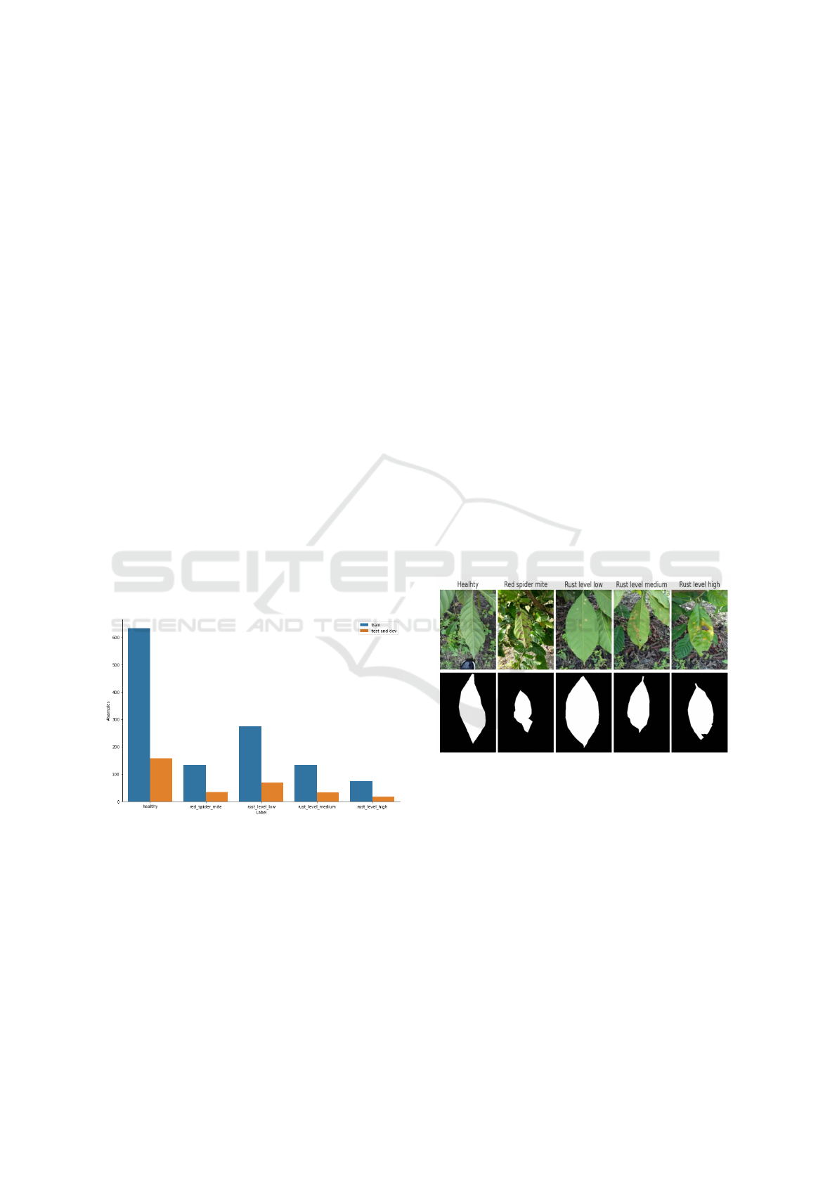
3.3 Split

The initial dataset is randomly split into train, devel-

opment (dev), and test sets as shown in Figure 1. The

split is done as follows: 80% goes to the train set, with

the rest of 20% being split equally between the dev

and test sets. After the split, the train and dev sets

are augmented together and then split back with an

80%-10% ratio. We do not augment the test set since

the model metrics computed on the test set must only

reﬂect the performance on data from the real input

distribution.

Figure 1: Statistics of the number of samples in the relabeled

dataset.

4 METHOD

4.1 Segmentation

As can be seen from the examples in Figure 2, the

backgrounds of the images are very random and do

not provide any additional information. Therefore, it

only makes sense to use masked images to train classi-

ﬁers. For training a classiﬁer, it is trivial to apply the

mask that comes with the image. Unfortunately, the

issue is for the examples that do not already come seg-

mented. The segmentation problem involves learning

a mapping from an input distribution to the distribu-

tion that represents the mask of the inputs. Because of

the pairwise nature of the segmentation problem, the

pix2pix model (Isola et al., 2017) is the perfect ﬁt for

it. Furthermore, pix2pix is based on the U-Net archi-

tecture, which is state of the art in image segmentation

(Siddique et al., 2021). The pix2pix model was thus

trained on image-mask pairs from the RoCoLe dataset.

To improve the quality of the predicted segmenta-

tion masks, online augmentation was also used to crop

and ﬂip the image randomly. After training, the mask

was inferred for each image in the dataset and then ap-

plied to the image to only contain the area of interest,

namely the leaf in the foreground. The reason segmen-

tation of the dataset is done using the trained pix2pix

model and not using the already provided masks is

because the inferred masks are slightly different from

the provided ones. Training a classiﬁer on images seg-

mented with the provided masks but segmenting the

test images with pix2pix will affect the quality of the

predictions as the input distribution for the classiﬁer

will be slightly different.

Figure 2: Examples of rescaled images from each class and

the associated masks.

4.2 Ofﬂine Augmentations

In order to alleviate the class imbalance, image gener-

ation was used to supplement the less frequent classes,

thus making the dataset perfectly balanced. The class

frequencies show that the healthy class is the most fre-

quent. This means that it can augment the other classes

by transferring the style of the images with diseased

leaves onto the images with healthy leaves. The cycle-

generative adversarial network (CycleGAN) model

(Zhu et al., 2017) has been proven to be effective for

style transfer tasks (Liu et al., 2020). Also, CycleGAN

Evaluating Data Augmentation Techniques for Coffee Leaf Disease Classiﬁcation

551

is a good ﬁt for the augmentation task since it does

not require paired inputs and works just as well with

unpaired inputs, which is the case for the augmentation

task.

In addition to learning the mapping from the source

domain

to the target domain

, CycleGAN also

learns the inverse mapping from the target domain to

the source domain (Zhu et al., 2017). In this sense,

two generators and two discriminators are used, one

of each type for each mapping:

and

for the di-

rect mapping

G : X → Y

, as well as

and

for the

inverse mapping

F : Y → X

. Furthermore, CycleGAN

introduces another objective, called cycle consistency

loss, in addition to the classic GAN objectives (Good-

fellow et al., 2014). Intuitively, this novel objective

uses the L1 norm to enforce the consistency of the in-

verse mapping, canceling the direct mapping, as shown

in Eq. (1).

cyc

(G, F) = E

x∼p

data

(x)

[||F(G(x)) − x||

+ E

y∼p

data

(y)

[||G(F(y)) − y||

] (1)

When passing an image from

through generator

or an image from

through generator

, the out-

put is expected to be the same provided image since

the input already comes from the output distribution.

Therefore, a second regularization loss called the iden-

tity loss is used to constrain the model. This loss uses

the same L1 norm as the cycle consistency loss and

can be expressed through Eq. (2).

identity

(G, F) = E

x∼p

data

(x)

[||F(x) − x||

+ E

y∼p

data

(y)

[||G(y) − y||

] (2)

By combining the identity and cycle consistency

losses with the standard GAN objectives, the ﬁnal loss

becomes as described by Eq. (3).

L (G, F, D

, D

) = L

GAN

(G, D

, X, Y )+

+ L

GAN

(F, D

, Y, X ) + λ

cyc

(G, F)+

+ λ

identity

(G, F) (3)

Therefore, we train the CycleGAN model on our

dataset of segmented images for each combination

of healthy and diseased classes. This means that four

CycleGAN models were trained in total. After training,

the models were used on every segmented image of the

healthy class to generate its diseased counterpart. The

dataset was augmented using those generated diseased

images by supplementing every diseased class such

that the number of samples in each class is equal. For

this, the required number of images was randomly

picked from the generated images.

4.3 Online Augmentations

During training, online augmentation of the dataset

was also tested. The most basic augmentations that

have been tested are horizontal and vertical ﬂips, as

well as random rotations. Therefore, an image is ro-

tated with a random angle between 0 and 180 degrees,

after which random horizontal and vertical ﬂips are

applied with a probability of 25% each.

More advanced techniques include MixUp (Zhang

et al., 2018), CutMix (Yun et al., 2019), Cutout (De-

Vries and Taylor, 2017), and FMix (Harris et al., 2020).

These augmentations are applied during the batching

process so that the training dataset will differ with

each epoch. For the batched augmentations, there is a

50% probability that the augmentation will be applied;

otherwise, the batch is left unmodiﬁed. Furthermore,

all batched augmentations use a random parameter

sampled from the beta distribution each time the aug-

mentation is applied. For FMix, the beta distribution’s

and

parameters are set to 1, while for the other

batched augmentations, both parameters are set to 0.8.

With CutMix and Cutout, the square that is cut out

is chosen to have the center at least one-quarter away

from the edge of the image, as most images have the

leaf centered in the middle of the image.

4.4 Classiﬁcation Models

After segmentation and augmentation, the dataset

is ready for training classiﬁcation models. Thus,

Transformer-based architectures (i.e., ViT (Dosovit-

skiy et al., 2020) and CvT (Wu et al., 2021)) were

tested using different hyperparameters, sizes, and aug-

mentation techniques. In order to compare these mod-

els to convolutional state-of-the-art models, ResNet

was tested in some scenarios.

5 EXPERIMENTAL SETUP

5.1 Performance Metrics

For model evaluation, macro-averaging was used to

combine accuracy, precision, recall, and F1-score bi-

nary classiﬁcation metrics into multiclass metrics.

Apart from the initial ViT and ResNet tests, all

tests also feature the top-k accuracy metric. Top-k

accuracy means that when calculating the accuracy

score, a prediction is considered accurate if any of the

top-k outputs with the highest conﬁdence is correct.

For testing, the top-2 accuracy was used in addition to

the classic accuracy metric.

ICAART 2024 - 16th International Conference on Agents and Artiﬁcial Intelligence

552

5.2 Hyperparameters

5.2.1 Pix2pix Setup

The pix2pix model was trained using the Adam opti-

mizer (Kingma and Ba, 2014) with a learning rate of

2 ∗ 10

−4

and the momentum parameters

and

set

to 0.5 and 0.999, respectively. These parameters are

the same as in the pix2pix paper (Isola et al., 2017).

Other parameters taken from the paper are the batch

size of 1, a value shown to work best for the pix2pix

model, and the L1 loss weight,

, set to 100. For the

discriminator, we used the PatchGAN (Li and Wand,

2016; Isola et al., 2017) of output size 30x30. The

model was trained on the whole dataset for 25 epochs.

5.2.2 CycleGAN Setup

For training the CycleGAN models, the Adam opti-

mizer was used along with the same learning rate, mo-

mentum parameters, and batch size as for the pix2pix

model. The weights for the cycle consistency loss and

identity loss were also taken from the CycleGAN paper

(Zhu et al., 2017), speciﬁcally from the “Monet paint-

ings to photos” experiment, and were set to 10 and 5,

respectively. From an architectural point of view, the

generator with nine residual blocks from the paper was

used, along with the 70x70 PatchGAN discriminator,

also from the paper (Zhu et al., 2017). Each model

was trained on the whole segmented dataset for 100

epochs.

5.2.3 Classiﬁcation Model Setup

All models were trained using a batch size of 32, with a

few exceptions where batch sizes of 16 were used due

to limited resources. The Adam optimizer was used,

along with a learning rate scheduler that multiplies the

learning rate by 0.25 every 15 epochs.

6 QUANTITATIVE RESULTS

6.1 Results for Ofﬂine Augmentations

Initially, we tested a ViT-small model with a patch size

of 16 and an input size of 224. The tests aim to com-

pare different models and augmentation techniques, so

the ﬁrst tests involve ﬁnding the optimum hyperparam-

eters at which to train the following models. Therefore,

the model is ﬁrst tested with and without dropout and

learning rates of 0.001 and 0.0002 for 50 epochs to

observe how hyperparameters affect the scores and the

evolution of train and dev losses.

The Augmentations Improve Performance in

Almost All Cases. As can be observed from Ta-

ble 1, the scores in most cases are higher when the

model is trained on the augmented dataset than the

non-augmented dataset. In the case of the ﬁfth and

sixth rows, the model has higher accuracy when trained

on the non-augmented dataset, but all the other scores

are low. The explanation is that the model overﬁts

the most frequent class because of the imbalanced na-

ture of the non-augmented dataset. However, for the

third and fourth rows, all the scores are higher for the

non-augmented model than all the others. As the differ-

ences are not that big, this anomaly can be explained

by the small dimension of the test set.

The ViT-Small Model Performs Better When

Trained Using a Lower Learning Rate. In Ta-

ble 1, in the case of no dropout and a learning rate of

0.001, the model presents worse performance on both

augmented and non-augmented datasets compared to

the cases when a learning rate of 0.0002 is used. This

means the lower learning rate is the correct choice,

as the model presents better learning abilities regard-

less of the dataset. Another observation in our tests

is that introducing dropout reduces overﬁtting mostly

on the augmented dataset, with the losses on the non-

augmented dataset remaining almost unchanged. Us-

ing a learning rate of 0.0002 and enabling dropout, the

overﬁtting on the augmented dataset almost disappears,

while it is greatly improved on the non-augmented

dataset.

The ResNet-50V2 and ResNet-101V2 models were

tested to compare how augmentation affects traditional

convolutional neural networks. Like the ViT, these

models are pre-trained on the ImageNet datasets (Deng

et al., 2009). A learning rate of 0.001 was used to test

both augmented and non-augmented datasets, while

all other settings were kept as before.

Bigger Models Encourage Overﬁtting. In Table

2, it can be noticed how ResNet performs worse in

the case of the bigger model, as the higher number

of parameters worsens overﬁtting. Furthermore, per-

formance is better on the augmented dataset for both

versions of ResNet, as the larger dataset discourages

overﬁtting.

ViT Has Better Performance Than ResNet.

When comparing the scores of the ViT-small with en-

abled dropout, augmentation, and a learning rate of

0.0002 to the ResNet-50V2 model with augmentation,

it can be observed that the Transformer-based model

performs better compared to the convolutional-based

model.

Evaluating Data Augmentation Techniques for Coffee Leaf Disease Classiﬁcation

553

Table 1: ViT-small scores for different combinations of hyperparameters.

Dropout Augmented Learning rate Accuracy Precision Recall F1

No Yes 0.001 64.1 54.4 56.9 55.0

No No 0.001 51.9 32.3 32 32.1

No Yes 0.0002 73.1 58.5 54.9 55.7

No No 0.0002 75.0 61.6 58.3 59.4

Yes Yes 0.001 57.1 42.3 43.5 42.0

Yes No 0.001 59.6 36.2 36.6 36.2

Yes Yes 0.0002 73.7 59.1 56.5 57.2

Yes No 0.0002 64.7 47.3 47.1 46.3

Table 2: ResNet scores for different variants and augmentations.

Model Augmented Accuracy Precision Recall F1

ResNet-50V2 Yes 69.2 48.7 47.9 47.7

ResNet-50V2 No 62.8 43.8 44.5 43.9

ResNet-101V2 Yes 61.5 43.6 42.3 42.6

ResNet-101V2 No 48.7 31.9 31.3 31.5

By analyzing the loss evolution of the models, it

could be noticed how the models started overﬁtting

mostly around 20 to 30 epochs. For this reason, all

tests described from now on will be done using 25

epochs. Regarding the other hyperparameters, enabled

dropout, a learning rate of 0.0002, and the augmented

dataset will be used. Until another model is tested, the

ViT-small model will be used.

In order to further test how well the synthetically

generated data captures the distribution of the real data,

we compared the Train on Real - Test on Real (TRTR),

Train on Real - Test on Synthetic (TRTS), Train on

Synthetic - Test on Real (TSTR), and Train on Syn-

thetic - Test on Synthetic (TSTS) scenarios (Fekri et al.,

2019). As the names suggest, these methods train and

test the model on combinations of either the original

dataset with real images or a dataset consisting of only

synthetic images with no real images in the augmented

classes. The synthetic data was thus extracted and split

into train, dev, and test using the same ratios as before.

Synthetic Data Poorly Captures the Distribution of

the Real Data. Table 3 shows how, to a certain

extent, the synthetic data captures the distribution of

the real data rather poorly. The discrepancy between

TRTR and TSTS especially shows this. The model

performs much better on synthetic data and learns by

overﬁtting the speciﬁc properties of each generated

class. As there is still one real class among the syn-

thetic images, the healthy class, as well as all other

synthetic classes being generated with different trained

instances of CycleGAN, the model learns to distin-

guish between the classes by learning the different

footprints left in the generated images.

Models Trained Only on Synthetic Data General-

ize Poorly to Real Data. The slight difference

between TRTR and TRTS shows how a model trained

on real data generalizes just as well to synthetic data,

as the model learns the actual distribution without

overﬁtting. The poor performance of TSTR compared

to TSTS further emphasizes how the model overﬁts

speciﬁc properties in the synthetic data and does not

generalize well to real data.

6.2 Results for Online Augmentations

Online Augmentations Improve Performance in Al-

most All Cases. It can be observed in Table 4 how,

with a few exceptions, online augmentations further

improve the performance when compared to the equiv-

alent conﬁguration in Table 1, speciﬁcally the second

to last row. One of the exceptions is Cutout, which has

no other augmentations.

Cutout with No Augmentations Offers the Worst

Performance. Because the segmented images

have most pixels set to 0, cutting out additional parts of

the image erases essential information. Adding other

augmentations seems to counteract this, as the Cutout

model with random rotations and ﬂips is among the

better-performing models.

FMix Features the Best All-Around Performance.

CutMix and FMix have similar performances, with

FMix taking the lead, especially when adding rotations

and ﬂips. Rotations and ﬂips seem to improve all

metrics except accuracy, while batched augmentations

have more of an effect on the standard accuracy metric.

Finally, we tested the CvT model (Wu et al., 2021)

on the augmented dataset, non-augmented dataset, and

the various combinations of online augmentations also

tested up until now. By analyzing the loss evolution,

we observed that CvT is more prone to overﬁtting,

ICAART 2024 - 16th International Conference on Agents and Artiﬁcial Intelligence

554

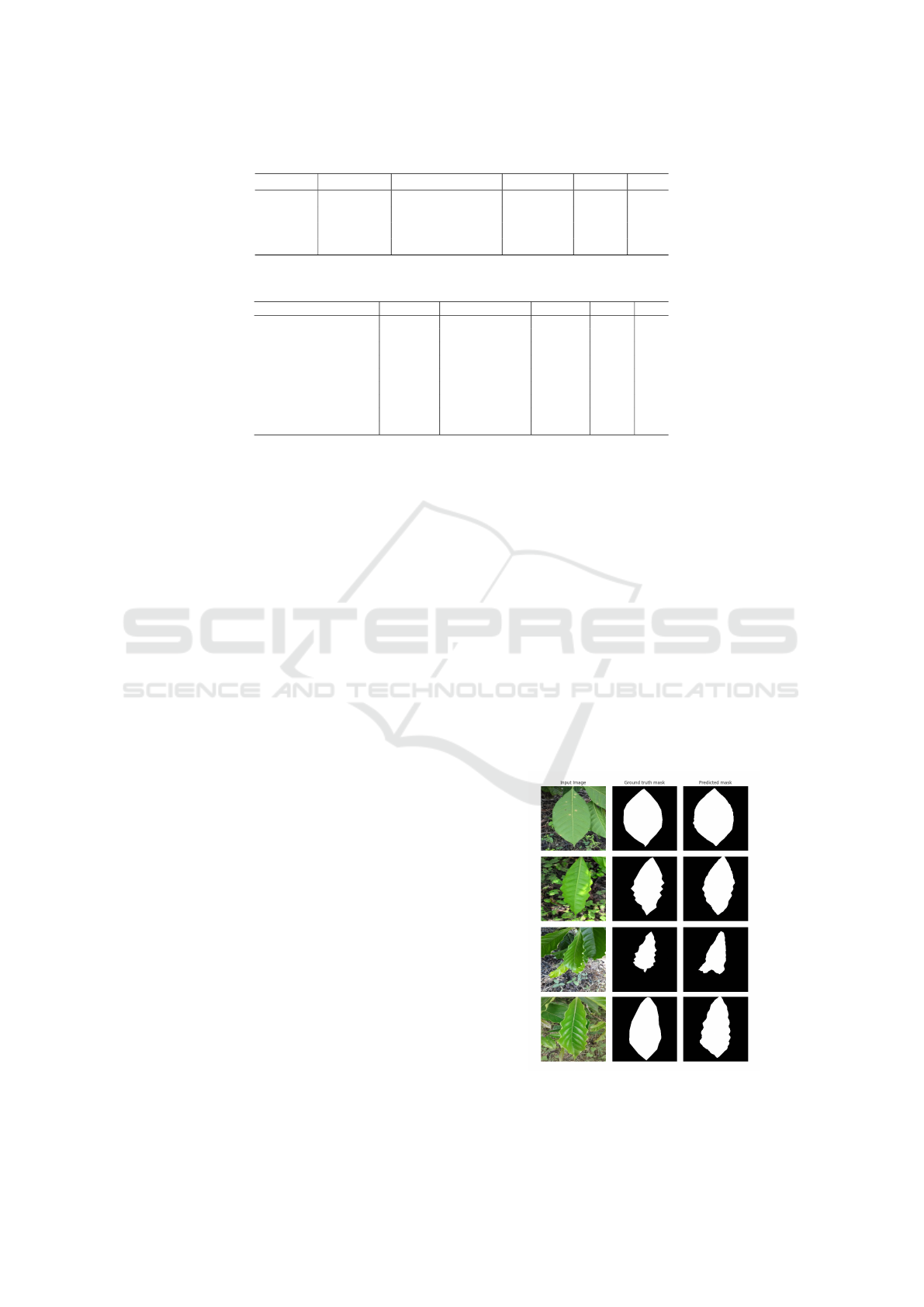
Table 3: ViT-small scores for TRTR, TRTS, TSTR, and TSTS.

Method Accuracy Top-2 Accuracy Precision Recall F1

TRTR 62.8 86.5 45.9 45.7 44.1

TRTS 62.3 84.0 60.1 55.7 55.4

TSTR 55.1 76.3 34.2 30.6 29.0

TSTS 96.9 99.6 97.1 96.2 96.6

Table 4: ViT-small scores for different online augmentations.

Augmentation Accuracy Top-2 Accuracy Precision Recall F1

Rotation+Flips 73.7 91.7 68.3 65.1 62.7

MixUp 73.7 88.5 60.1 57.4 57.0

CutMix 76.3 88.5 62.9 59.9 59.7

Cutout 69.2 89.1 53.7 51.6 51.3

FMix 74.4 89.7 64.2 57.8 59.1

Rotation+Flips+MixUp 69.9 93.6 52.2 50.1 49.4

Rotation+Flips+CutMix 73.7 88.5 66.4 57.5 59.3

Rotation+Flips+Cutout 76.3 92.3 68.1 65.5 63.3

Rotation+Flips+FMix 77.6 91.0 71.6 67.1 67.7

being a bigger model than ViT. The augmented dataset

helped with overﬁtting, as did the augmentations with

random rotations and ﬂips. The choice of batched

augmentation did not impact overﬁtting much, but

CutMix and FMix had slightly better performance in

that aspect.

CvT Has Similar Performance to ViT. As seen

in Table 5, the performances of CvT are similar to ViT,

with rotation and ﬂip augmentations making the model

carry out better. In the case of CvT, the versions where

Cutout is used have similar performance and perform

better than the other batched augmentations. While

ViT favored CutMix over MixUp, the performances

are ﬂipped with CvT, such that CutMix outperforms

MixUp. FMix seems to be the most robust, with its

performance having smaller ﬂuctuations than the rest

of the batched augmentations, regardless of the model

or the other online augmentations used. Using the non-

augmented dataset has the same performance impact

on CvT as it had on ViT.

7 QUALITATIVE RESULTS

7.1 Pix2pix Examples

Predicted Masks Are Smoother Than Hand-Drawn

Masks. As can be seen in the ﬁrst and second ex-

amples of Figure 3, the predicted mask is smoother

around the edges compared to the ground truth mask,

albeit less close to the outline of the leaf. The fourth

example shows that the model could generate a mask

that surpasses the ground truth in the correct condi-

tions.

Predicted Masks Sometimes Include Background

Leaves. The third image shows how certain back-

ground leaves hinder the model’s ability to ﬁnd an

outline that follows the exact shape of the leaf, out-

putting a smoother segmentation instead. Therefore,

in areas where the outline is less visible, the model

also includes the background leaves when performing

segmentation.

The Model Has Trouble Segmenting Leaves Against

Speciﬁc Backgrounds. Because the pix2pix

model was trained on images that mostly contain back-

grounds of other leaves combined with grass and dirt, it

has trouble segmenting images of leaves taken against

backgrounds such as asphalt and concrete. Surpris-

ingly, the model is good at segmenting images of

leaves taken against plain or solid color backgrounds.

Figure 3: Examples of pix2pix predicted masks compared to

the ground truth masks.

Evaluating Data Augmentation Techniques for Coffee Leaf Disease Classiﬁcation

555

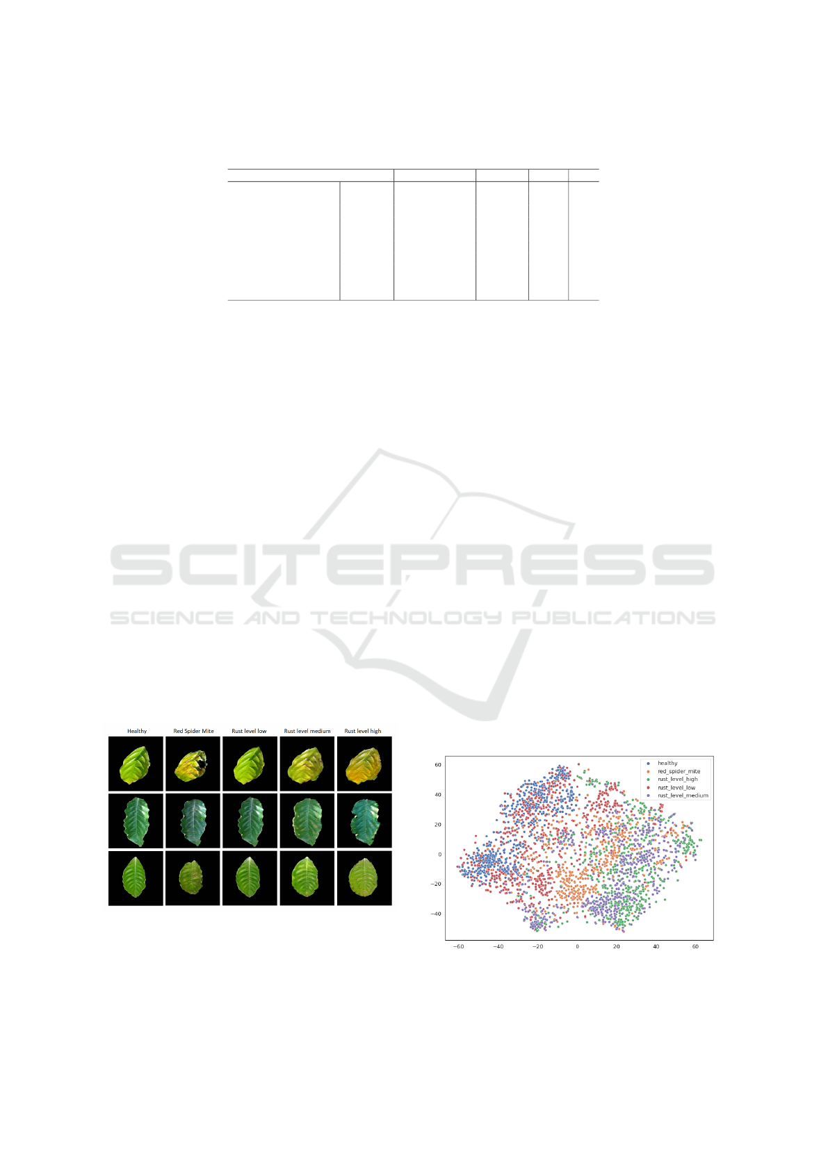
Table 5: CvT scores for the ofﬂine augmented dataset (ﬁrst row), the non-augmented dataset (second row), and the augmented

dataset with combinations of online augmentations (from third to last row).

Augmentation Accuracy Top-2 Accuracy Precision Recall F1

Augmented 76.3 91.7 62.1 58.9 60.2

Non-augmented 59.0 80.8 43.4 44.2 43.4

MixUp 75.0 89.7 55.6 53.6 54.1

CutMix 71.2 84.6 55.9 54.3 54.8

Cutout 75.0 92.9 61.1 60.6 60.6

FMix 75.0 85.9 60.5 60.8 59.8

Rotation+Flips+MixUp 76.3 89.7 63.2 62.6 62.8

Rotation+Flips+CutMix 75.0 91.0 58.9 60.4 58.9

Rotation+Flips+Cutout 78.2 92.9 66.1 64.3 63.4

Rotation+Flips+FMix 76.9 91.0 61.5 63.0 61.0

7.2 CycleGAN Examples

Some Synthetic Images Contain Noisy Holes. As

shown in the ﬁrst example of Figure 4, the generated

red_spider_mite image features a big hole in the leaf.

While the hole is an excellent example of leaf dam-

age, there is also a lot of noise surrounding it, which

decays the quality of the sample. Better-looking hole

examples are found in the high rust-level image gener-

ated from the second healthy leaf, the synthetic image

featuring small holes around the edges of the leaf.

The Low Rust-Level Synthetic Images Feature Al-

most No Discernible Modiﬁcations. For the low

rust level, there is little discernible difference between

the healthy and diseased images. This might be be-

cause this level of rust has a minimal impact on the

appearance of the leaf, making it look almost identical

to a healthy leaf in most cases. In comparison, the

medium and high levels of rust have the most visible

effects. As expected, the ﬁrst and third examples show

more severe rust stains for the high level than for the

medium level, while the second example shows more

holes.

Figure 4: Examples of diseased leaf images generated from

healthy leaf images.

7.3 T-SNE Visualizations

In order to show how the generated diseased leaf im-

ages are close to the actual images in the input distri-

bution space, latent features are ﬁrst extracted from

the images by passing them through a ViT. This vision

Transformer is pre-trained on the ImageNet-21k and

ImageNet-1k datasets (Deng et al., 2009), so it should

extract distinctive features out of the leaf images with-

out prior knowledge about the input distribution. In

order to visualize those latent features, the t-distributed

stochastic neighbor embedding (t-SNE) dimensional-

ity reduction technique (Hinton and Roweis, 2002) is

used.

In Figure 5, it is easy to notice how the different

classes are each spread into their clusters, with the

clusters also overlapping each other a bit. This is ex-

pected from a model pre-trained on a generic image

dataset without prior knowledge of the plant leaf clas-

siﬁcation task. It can still be observed how there are

no evident outliers for any class, with the synthetic

images seemingly blending into the real images.

In Figure 6, for the most part, the synthetic image

representations surround the real images representa-

tions, except for the red_spider_mite class, where the

real and synthetic images overlap almost perfectly.

Figure 5: 2D t-SNE representations of each class’s images,

both synthetic and real.

ICAART 2024 - 16th International Conference on Agents and Artiﬁcial Intelligence

556

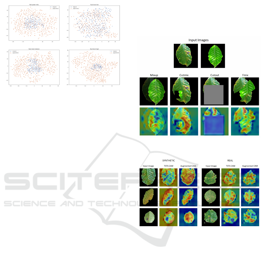
Figure 6: 2D t-SNE visualizations of each class, comparing

real and synthetic images.

7.4 CAM Visualizations

Models Trained with Certain Online Augmenta-

tions Focus Better on the Critical Parts of Leaves.

For the MixUp strategy, the model focuses more on the

area where the two images overlap, and there are no

rust spots (see Figure 7). Interestingly, the big rust re-

gion is mainly ignored, with the model focusing more

on the small rust spots on the left side of the rusty

leaf. For CutMix, the model learned to ignore the ar-

eas that encompass the transitions from one image to

another while also focusing on the essential elements

in both images. With Cutout, even when a big area

is cut out in the image, the model learns to ignore it

and focuses instead on the unobstructed regions. FMix

CAM is similar to CutMix CAM, the model ignoring

the transitions, especially in regions where one image

transitions to the background of the other image.

Models Trained On Synthetic Data Focus More

on the Background and Edges of Leaves. The

CAMs in Figure 8 show how the model trained on

the synthetic dataset focuses the most on the edges

of the leaves, where more artifacts were left by the

CycleGAN model when generating the images. Also,

the TSTS model seems to focus surprisingly much

on the background, which can be explained because

the CycleGAN model leaves noise in the background

of the generated image. The model trained on the

augmented dataset focuses the most on areas where

the leaf is affected by rust.

Models Trained Using Online Augmentations Focus

on the Image as a Whole. By comparing the vi-

sualizations in Figure 7 to the visualizations in Figure

8, it can be observed that the models trained using on-

line augmentations direct their attention more toward

the background of the image compared to the model

trained without online augmentations. This is because

the models trained using online augmentations learn to

focus on the image as a whole, not only on the center

part.

Figure 7: CAM visualizations for batched augmentation

techniques.

Figure 8: CAM visualizations for synthetic (left) and real

(right) for the TSTS model (TSTS CAM) and a model trained

normally on the augmented dataset (Augmented CAM). All

images are part of the rust_level_high class.

8 CONCLUSIONS AND FUTURE

WORK

This paper presented a deep learning pipeline for

the task of leaf disease classiﬁcation on the RoCoLe

dataset. Consequently, image leaf segmentation was

performed using a pix2pix model, and CycleGAN was

used to augment the diseased classes in the dataset.

Also, Transformer-based image classiﬁcation models

were trained on the augmented dataset using various

online augmentations.

This approach of using augmentations combined

with Transformer models increased the classiﬁcation

performance compared to approaches using convolu-

Evaluating Data Augmentation Techniques for Coffee Leaf Disease Classiﬁcation

557

tional models or without augmentations. Even though

the results of the TRTR, TRTS, TSTR, and TSTS sce-

narios showed that the synthetic data only vaguely

captures the distribution of the real data, the increased

performance of the models trained on the augmented

dataset proved that the CycleGAN augmentations were

helpful.

The presented approach can still be improved, with

better alternatives being viable in most parts of the

architecture. Therefore, the main improvement that

can be implemented is the use of the StarGAN (Choi

et al., 2018) multi-domain image translation model for

augmenting the RoCoLe dataset. This approach would

beneﬁt from needing only one model to be trained for

augmenting all diseased classes. Other GAN varia-

tions can also be tested, such as the Wasserstein GAN

(Arjovsky et al., 2017), which has proven more stable

than other GANs.

The leaf segmentation could also be improved

by using semantic segmentation (Tassis et al., 2021).

However, this would increase computational costs. A

cheaper alternative would be to implement semantic

segmentation using either the previously presented

CAM method or the better GradCAM variant (Sel-

varaju et al., 2017).

Finally, a Swin Transformer (Liu et al., 2021) can

be used as a classiﬁer instead of the ViT or CvT. An-

other alternative would be to use vision-language mod-

els (Yu et al., 2022), which are the current state of

the art in image classiﬁcation. Models like the con-

trastive captioner (Yu et al., 2022) use encoder-decoder

architectures to learn captions for images, so the en-

coder could be ﬁne-tuned to classify images from the

RoCoLe dataset.

ACKNOWLEDGEMENTS

This work was supported by GNAC ARUT 2023.

REFERENCES

Arjovsky, M., Chintala, S., and Bottou, L. (2017). Wasser-

stein generative adversarial networks. In Interna-

tional conference on machine learning, pages 214–223.

PMLR.

Brahimi, M., Boukhalfa, K., and Moussaoui, A. (2017).

Deep learning for tomato diseases: classiﬁcation and

symptoms visualization. Applied Artiﬁcial Intelligence,

31(4):299–315.

Choi, Y., Choi, M., Kim, M., Ha, J.-W., Kim, S., and Choo,

J. (2018). Stargan: Uniﬁed generative adversarial net-

works for multi-domain image-to-image translation.

In Proceedings of the IEEE conference on computer

vision and pattern recognition, pages 8789–8797.

Dawod, R. G. and Dobre, C. (2021). Classiﬁcation of

sunﬂower foliar diseases using convolutional neural

network. In 2021 23rd International Conference on

Control Systems and Computer Science (CSCS), pages

476–481. IEEE.

Dawod, R. G. and Dobre, C. (2022a). Automatic segmen-

tation and classiﬁcation system for foliar diseases in

sunﬂower. Sustainability, 14(18):11312.

Dawod, R. G. and Dobre, C. (2022b). Resnet interpretation

methods applied to the classiﬁcation of foliar diseases

in sunﬂower. Journal of Agriculture and Food Re-

search, 9:100323.

Dawod, R. G. and Dobre, C. (2022c). Upper and lower leaf

side detection with machine learning methods. Sensors,

22(7):2696.

Deng, J., Dong, W., Socher, R., Li, L.-J., Li, K., and Fei-Fei,

L. (2009). Imagenet: A large-scale hierarchical image

database. In 2009 IEEE conference on computer vision

and pattern recognition, pages 248–255. Ieee.

DeVries, T. and Taylor, G. W. (2017). Improved regular-

ization of convolutional neural networks with cutout.

arXiv preprint arXiv:1708.04552.

Ding, S., Wang, J., Li, J., and Shi, J. (2023). Multi-scale

prototypical transformer for whole slide image classiﬁ-

cation. In International conference on medical image

computing and computer-assisted intervention, pages

602–611. Springer.

Dosovitskiy, A., Beyer, L., Kolesnikov, A., Weissenborn,

D., Zhai, X., Unterthiner, T., Dehghani, M., Minderer,

M., Heigold, G., Gelly, S., et al. (2020). An image is

worth 16x16 words: Transformers for image recogni-

tion at scale. In International Conference on Learning

Representations.

Echim, S.-V., T

aiatu, I.-M., Cercel, D.-C., and Pop, F. (2023).

Explainability-driven leaf disease classiﬁcation using

adversarial training and knowledge distillation.

Faisal, M., Leu, J.-S., and Darmawan, J. T. (2023). Model

selection of hybrid feature fusion for coffee leaf disease

classiﬁcation. IEEE Access.

Fekri, M. N., Ghosh, A. M., and Grolinger, K. (2019). Gen-

erating energy data for machine learning with recurrent

generative adversarial networks. Energies, 13(1):130.

Goodfellow, I., Pouget-Abadie, J., Mirza, M., Xu, B., Warde-

Farley, D., Ozair, S., Courville, A., and Bengio, Y.

(2014). Generative adversarial nets. Advances in neural

information processing systems, 27.

Harris, E., Marcu, A., Painter, M., Niranjan, M., Prügel-

Bennett, A., and Hare, J. (2020). Fmix: Enhanc-

ing mixed sample data augmentation. arXiv preprint

arXiv:2002.12047.

He, K., Gkioxari, G., Dollár, P., and Girshick, R. (2017).

Mask r-cnn. arxiv e-prints, page. arXiv preprint

arXiv:1703.06870.

He, K., Zhang, X., Ren, S., and Sun, J. (2016). Deep resid-

ual learning for image recognition. In Proceedings of

the IEEE conference on computer vision and pattern

recognition, pages 770–778.

ICAART 2024 - 16th International Conference on Agents and Artiﬁcial Intelligence

558

Hinton, G. E. and Roweis, S. (2002). Stochastic neighbor

embedding. In Becker, S., Thrun, S., and Obermayer,

K., editors, Advances in Neural Information Process-

ing Systems, volume 15. MIT Press.

Isola, P., Zhu, J.-Y., Zhou, T., and Efros, A. A. (2017). Image-

to-image translation with conditional adversarial net-

works. In Proceedings of the IEEE conference on

computer vision and pattern recognition, pages 1125–

1134.

Kamal, K., Yin, Z., Wu, M., and Wu, Z. (2019). Depthwise

separable convolution architectures for plant disease

classiﬁcation. Computers and electronics in agricul-

ture, 165:104948.

Kim, Y. (2014). Convolutional neural networks for sentence

classiﬁcation. In Proceedings of the 2014 Conference

on Empirical Methods in Natural Language Processing

(EMNLP). Association for Computational Linguistics.

Kingma, D. P. and Ba, J. (2014). Adam: A

method for stochastic optimization. arXiv preprint

arXiv:1412.6980.

Krizhevsky, A., Sutskever, I., and Hinton, G. E. (2017).

Imagenet classiﬁcation with deep convolutional neural

networks. Communications of the ACM, 60(6):84–90.

Li, C. and Wand, M. (2016). Combining markov random

ﬁelds and convolutional neural networks for image

synthesis. In Proceedings of the IEEE conference on

computer vision and pattern recognition, pages 2479–

2486.

Liu, C., Chang, X., and Shen, Y.-D. (2020). Unity style

transfer for person re-identiﬁcation. In Proceedings

of the IEEE/CVF conference on computer vision and

pattern recognition, pages 6887–6896.

Liu, Z., Lin, Y., Cao, Y., Hu, H., Wei, Y., Zhang, Z., Lin,

S., and Guo, B. (2021). Swin transformer: Hierar-

chical vision transformer using shifted windows. In

Proceedings of the IEEE/CVF international conference

on computer vision, pages 10012–10022.

Lungu-Stan, V.-C., Cercel, D.-C., and Pop, F. (2023).

Skindistilvit: Lightweight vision transformer for skin

lesion classiﬁcation. In International Conference on

Artiﬁcial Neural Networks, pages 268–280. Springer.

Mohameth, F., Bingcai, C., and Sada, K. A. (2020). Plant

disease detection with deep learning and feature ex-

traction using plant village. Journal of Computer and

Communications, 8(6):10–22.

Mohanty, S. P., Hughes, D. P., and Salathé, M. (2016). Using

deep learning for image-based plant disease detection.

Frontiers in Plant Science, 7.

Nääs, I. A., Garcia, R. G., and Caldara, F. R. (2020). In-

frared thermal image for assessing animal health and

welfare. Journal of Animal Behaviour and Biometeo-

rology, 2(3):66–72.

Nam, M. G. and Dong, S.-Y. (2023). Classiﬁcation of com-

panion animals’ ocular diseases: Domain adversarial

learning for imbalanced data. IEEE Access.

Parraga-Alava, J., Cusme, K., Loor, A., and Santander, E.

(2019). Rocole: A robusta coffee leaf images dataset

for evaluation of machine learning based methods in

plant diseases recognition. Data in brief, 25:104414.

Rodriguez-Gallo, Y., Escobar-Benitez, B., and Rodriguez-

Lainez, J. (2023). Robust coffee rust detection us-

ing uav-based aerial rgb imagery. AgriEngineering,

5(3):1415–1431.

Ronneberger, O., Fischer, P., and Brox, T. (2015). U-

net: Convolutional networks for biomedical image

segmentation. In Medical Image Computing and

Computer-Assisted Intervention–MICCAI 2015: 18th

International Conference, Munich, Germany, October

5-9, 2015, Proceedings, Part III 18, pages 234–241.

Springer.

Selvaraju, R. R., Cogswell, M., Das, A., Vedantam, R.,

Parikh, D., and Batra, D. (2017). Grad-cam: Visual

explanations from deep networks via gradient-based

localization. In 2017 IEEE International Conference

on Computer Vision (ICCV), pages 618–626.

Siddique, N., Paheding, S., Elkin, C. P., and Devabhaktuni,

V. (2021). U-net and its variants for medical image

segmentation: A review of theory and applications.

Ieee Access, 9:82031–82057.

Simonyan, K. and Zisserman, A. (2015). Very deep con-

volutional networks for large-scale image recognition.

In 3rd International Conference on Learning Repre-

sentations (ICLR 2015). Computational and Biological

Learning Society.

Stauber, J., Lemaire, R., Franck, J., Bonnel, D., Croix,

D., Day, R., Wisztorski, M., Fournier, I., and Salzet,

M. (2008). Maldi imaging of formalin-ﬁxed parafﬁn-

embedded tissues: application to model animals of

parkinson disease for biomarker hunting. Journal of

Proteome Research, 7(3):969–978.

Sun, M., Huang, W., and Zheng, Y. (2023). Instance-aware

diffusion model for gland segmentation in colon histol-

ogy images. In International Conference on Medical

Image Computing and Computer-Assisted Intervention,

pages 662–672. Springer.

Szegedy, C., Liu, W., Jia, Y., Sermanet, P., Reed, S.,

Anguelov, D., Erhan, D., Vanhoucke, V., and Rabi-

novich, A. (2015). Going deeper with convolutions.

In Proceedings of the IEEE conference on computer

vision and pattern recognition, pages 1–9.

Tassis, L. M., de Souza, J. E. T., and Krohling, R. A. (2021).

A deep learning approach combining instance and se-

mantic segmentation to identify diseases and pests of

coffee leaves from in-ﬁeld images. Computers and

Electronics in Agriculture, 186:106191.

Thakur, P. S., Sheorey, T., and Ojha, A. (2023). Vgg-icnn: A

lightweight cnn model for crop disease identiﬁcation.

Multimedia Tools and Applications, 82(1):497–520.

Vaswani, A., Shazeer, N., Parmar, N., Uszkoreit, J., Jones,

L., Gomez, A. N., Kaiser, Ł., and Polosukhin, I. (2017).

Attention is all you need. Advances in neural informa-

tion processing systems, 30.

Wu, H., Xiao, B., Codella, N., Liu, M., Dai, X., Yuan, L.,

and Zhang, L. (2021). Cvt: Introducing convolutions to

vision transformers. In Proceedings of the IEEE/CVF

International Conference on Computer Vision, pages

22–31.

Yu, J., Wang, Z., Vasudevan, V., Yeung, L., Seyedhosseini,

M., and Wu, Y. (2022). Coca: Contrastive caption-

Evaluating Data Augmentation Techniques for Coffee Leaf Disease Classiﬁcation

559

ers are image-text foundation models. arXiv preprint

arXiv:2205.01917.

Yun, S., Han, D., Oh, S. J., Chun, S., Choe, J., and Yoo, Y.

(2019). Cutmix: Regularization strategy to train strong

classiﬁers with localizable features. In Proceedings of

the IEEE/CVF international conference on computer

vision, pages 6023–6032.

Zhang, H., Cisse, M., Dauphin, Y. N., and Lopez-Paz, D.

(2018). mixup: Beyond empirical risk minimization.

In International Conference on Learning Representa-

tions.

Zhao, H., Shi, J., Qi, X., Wang, X., and Jia, J. (2017). Pyra-

mid scene parsing network. In Proceedings of the IEEE

conference on computer vision and pattern recognition,

pages 2881–2890.

Zhou, B., Khosla, A., Lapedriza, A., Oliva, A., and Torralba,

A. (2016). Learning deep features for discriminative

localization. In Proceedings of the IEEE conference on

computer vision and pattern recognition, pages 2921–

2929.

Zhu, J.-Y., Park, T., Isola, P., and Efros, A. A. (2017).

Unpaired image-to-image translation using cycle-

consistent adversarial networks. In Proceedings of

the IEEE international conference on computer vision,

pages 2223–2232.

ICAART 2024 - 16th International Conference on Agents and Artiﬁcial Intelligence

560