Single-Class Instance Segmentation for Vectorization of Line Drawings

Rhythm Vohra

, Amanda Dash

and Alexandra Branzan Albu

University of Victoria, Canada

Keywords:

Segmentation, Visual Attention, Image Vectorization.

Abstract:

Images can be represented and stored either in raster or in vector formats. Raster images are most ubiquitous

and are deﬁned as matrices of pixel intensities/colours, while vector images consist of a ﬁnite set of geometric

primitives, such as lines, curves, and polygons. Since geometric shapes are expressed via mathematical equa-

tions and deﬁned by a limited number of control points, they can be manipulated in a much easier way than

by directly working with pixels; hence, the vector format is much preferred to raster for image editing and

understanding purposes. The conversion of a raster image into its vector correspondent is a non-trivial pro-

cess, called image vectorization. This paper presents a vectorization method for line drawings, which is much

faster and more accurate than the state-of-the-art. We propose a novel segmentation method that processes

the input raster image by labeling each pixel as belonging to a particular stroke instance. Our contributions

consist of a segmentation model (called Multi-Focus Attention UNet), as well as a loss function that handles

well infrequent labels and yields outputs which capture accurately the human drawing style.

1 INTRODUCTION

Images are rich sources of information which can be

stored in either raster or vector formats. Cameras use

sensors that capture the real-world scene in a grid

of photosensitive elements (with each of these ele-

ments corresponding to pixels in the image), and dig-

ital screens display images as an array of pixels. As

a result, most of the images available to us are stored

in raster format. Raster images have applications in

various contexts, including digital photography, print,

media, web designs, screens, and many others. Since

raster images consist of a ﬁxed number of pixels,

when zoomed-in or modiﬁed, the quality of the raster

image gets degraded, as shown in Figure 1.

A high-quality raster image may consist of thou-

sands to millions of pixels; thus raster images are dif-

ﬁcult to edit at a pixel level. Additionally, these im-

ages require ample storage space. Instead, images can

be compressed using various algorithms which reduce

the quality of raw raster images. A trade-off exists be-

tween a high compression ratio and a high-quality im-

age. Vector images are a more elegant solution to this

trade-off, as they use less storage space while main-

taining high image quality.

https://orcid.org/0009-0004-0071-0720

https://orcid.org/0000-0001-8654-1593

https://orcid.org/0000-0001-8991-0999

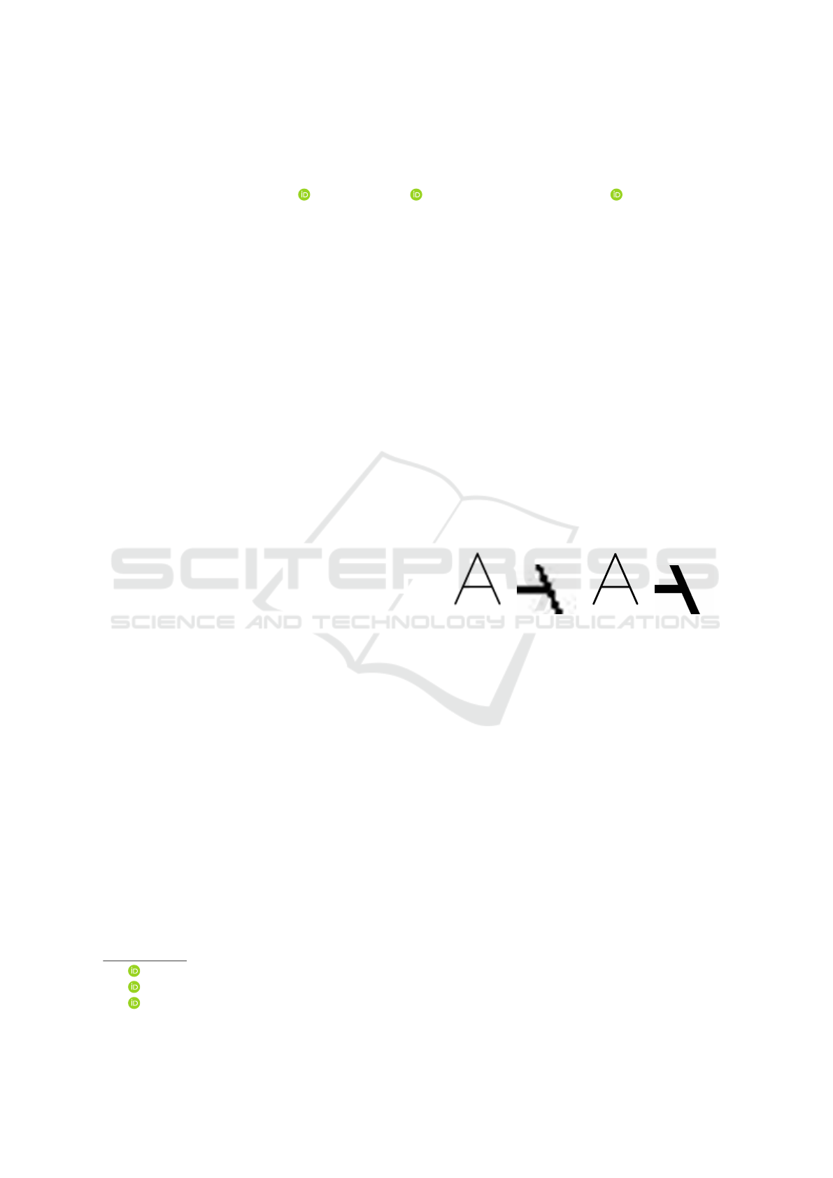
(a) (b) (c) (d)

Figure 1: Comparison between vector and raster images

when zoomed in; vector images maintain clean lines, while

raster images get blurred because of constraints in resolu-

tion. (a) Raster image, (b) Zoomed-in raster image, (c) Vec-

tor image, (d) Zoomed-in vector image.

Vector images are described by geometric primi-

tives such as curves and their control points. Bezier

curves are used most frequently; they are based on

Bernstein polynomials (de Casteljau, 1963), con-

structing smooth and continuous shapes. Vector im-

ages have phenomenal ﬂexibility because they can be

stretched, rotated, or scaled while not compromising

their clarity, just by changing the position of con-

trol points. Editing these mathematically described

shapes is much easier than editing pixels in a raster

image. The edited images maintain their sharpness

across a wide range of resolutions, a highly desirable

attribute (see Figure 1).

Graphical designers perform many drawings man-

ually, using a pen or stylus. As a result, there is

a signiﬁcant need for converting hand-drawn raster

images into vector formats. Commercial vectoriza-

tion tools such as InkSpace, CorelDRAW, and Ado-

Vohra, R., Dash, A. and Branzan Albu, A.

Single-Class Instance Segmentation for Vectorization of Line Drawings.

DOI: 10.5220/0012465900003660

Paper published under CC license (CC BY-NC-ND 4.0)

In Proceedings of the 19th International Joint Conference on Computer Vision, Imaging and Computer Graphics Theory and Applications (VISIGRAPP 2024) - Volume 3: VISAPP, pages

215-226

ISBN: 978-989-758-679-8; ISSN: 2184-4321

215

beTrace use manual tracing of the vector lines from

the raster drawings by a skilled user. However, this

manual tracing process is labour-intensive and time-

consuming.

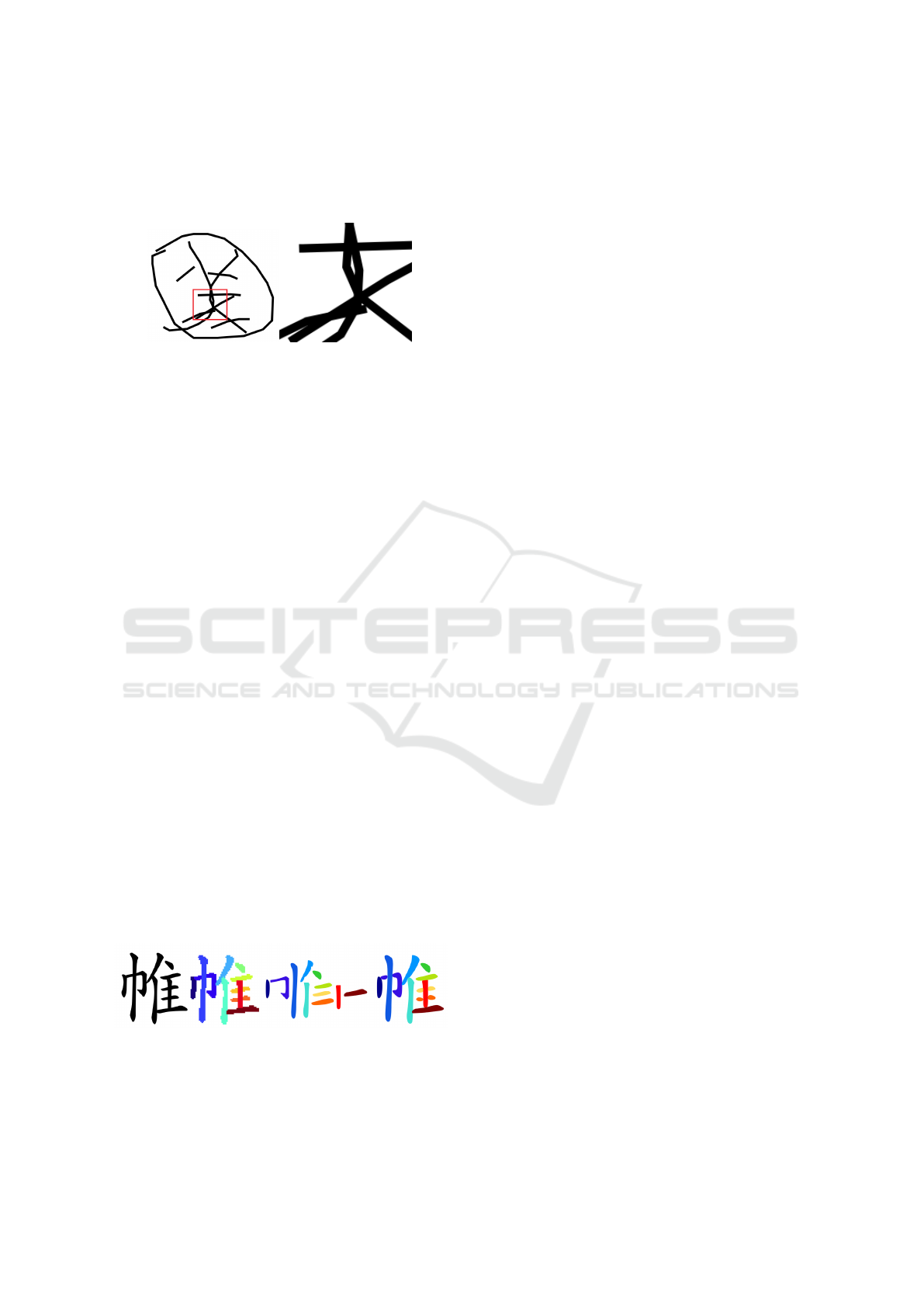
(a) (b)

Figure 2: (a) Example of an input image from our dataset

with red highlighted region zoomed in. (b) The zoomed-in

version of the input image depicts the overlapping regions,

emphasizing the importance of considering the global con-

text of the overall image to accurately identify which label

belongs to each stroke.

Our approach performs Single-Class Instance

Segmentation (SCIS), i.e., classiﬁcation of each

stroke individually, to convert hand-drawn strokes

(i.e. instances) from binary (one-class) raster images

into vector-based stroke representations. We propose

a segmentation method that processes the input raster

image by labeling each pixel as belonging to a partic-

ular stroke instance. The labelled regions in the out-

put of our segmentation model are separately vector-

ized using a commercial tool called Potrace (Selinger,

2003). The vectorized forms of all strokes are then

combined to form the ﬁnal vector image (see Figure

3).

Our contributions are two-fold:

1. We propose a novel segmentation model named

Multi-Focus Attention UNet (MFAU) that out-

performs a state-of-the-art method (Kim et al.,

2018), on several datasets using various perfor-

mance metrics.

2. We propose a novel loss function, the Margin-

Regularised Loss Function (MRLF) , that general-

izes well on less frequent labels in a highly imbal-

anced dataset. Our loss function also enables us

to generate outputs that are consistent with users’

drawing styles and with the perceptual grouping

principles of similarity, continuity and closure.

Figure 3: Vectorization by segmenting each stroke instance

of a line drawing. Left to Right: Grayscale raster image;

segmented output of raster image; instances separated and

vectorized, relative position is intentionally modiﬁed for vi-

sualization purposes; ﬁnal vectorized result.

The rest of this paper is organized as follows. Sec-

tion 2 presents a brief literature review on vectoriza-

tion of line drawings. Section 3 presents the pro-

posed segmentation model and loss function. Sec-

tion 4 discusses experimental results and compares

the proposed model with the state of the art. Section

5 draws conclusions and outlines future work direc-

tions.

2 RELATED WORK

This section discusses ﬁrst vectorization methods that

focus on detecting geometric primitives with tradi-

tional computer vision and image processing tech-

niques; next, we focus on recent deep-learning based

approaches.

Early works (Kultanen, 1990; Jimenez and

Navalon, 1982; Roosli and Monagan, 1996; Tombre

et al., 2000; Hilaire and Tombre, 2006) combined a

variety of image processing operators and techniques

such as thinning, thresholding, layering, contour ﬁnd-

ing, edge detection, curve ﬁtting, feature point extrac-

tion, Hough transform, and polygonal approximation.

(Dori, 1997) proposed an Orthogonal Zig-Zag

(OZZ) algorithm for vectorizing engineering draw-

ings that focuses on line recognition with improved

performance and with signiﬁcantly lower computa-

tional complexity with respect to the Hough Trans-

form. This algorithm detects lines in binary images

by using the same principle as the propagation of a

ray of light through optical ﬁber. The one-pixel wide

ray traverses the black pixels, treating them as a con-

ducting path. Whenever the ray encounters a white

pixel, its direction changes by 90

◦

. The ray therefore

collects information about the presence of lines, their

width, their start and end points, and enables skipping

junctions.

(Bartolo et al., 2007) proposed a technique to vec-

torize scribbled drawings for computer-aided design

(CAD) interpretation which is compatible with the

natural drawing habits of the user. They used Ga-

bor ﬁlters to simplify the scribbles, and then extracted

vector lines with a Kalman ﬁlter.

(Favreau et al., 2016) proposed the ﬁrst algorithm

that balances ﬁdelity to the raster input along with

simplicity of the output to generate an accurate and

compact number of curves via a global optimization

approach. Their algorithm’s robustness is shown on a

variety of drawings and human-made sketches.

Some vectorization techniques have matured

enough to be integrated in commercial tools. Po-

trace Inkscape (Selinger, 2003), Adobe Illustrator Im-

age Tracing (Wood, 2012), and CorelDraw (Bouton,

VISAPP 2024 - 19th International Conference on Computer Vision Theory and Applications

216

2014), focus on maintaining high visual accuracy and

quality during the vectorization process.

(Najgebauer and Scherer, 2019) introduced a

method that performs fast vectorization of line draw-

ings based on multi-scale second derivative detector

and inertia-based line tracing to improve accuracy at

junctions.

(Zhang et al., 2022) proposed a deep-learning

based semantic segmentation method for line vector-

ization of engineering drawings. They used a com-

bination of feature extraction, a non-local segmen-

tation algorithm based on dilated convolution and

self-attention module, and local rasterization. They

claimed robustness to typical line drawing problems

such as blurring and line breakage.

(Inoue and Yamasaki, 2019) introduced an in-

stance segmentation technique that is data-driven and

utilized deep networks to segment strokes based on

the global image context. They used a model based on

MaskRCNN (He et al., 2017) to perform instance seg-

mentation of hand drawings in a more efﬁcient way.

They proposed two modiﬁcations to the MaskRCNN

architecture: upsampling the masks generated from

the mask branch in order to detect ﬁner details, and a

post-processing for the correction of mismatched pix-

els.

(Kim et al., 2018) elegantly formulated the prob-

lem of vectorization as computing an instance seg-

mentation of the most likely set of paths that could

have created the input raster image. They trained a

pair of networks to help solve ambiguities in regions

where multiple path intersect and hence overlap. Both

networks take into account the global context of the

image, hence yielding a semantic vectorization.

We consider (Kim et al., 2018) as a state-of-the-

art approach in vectorization viewed as an instance

segmentation problem. Our approach proposes a dif-

ferent way of solving ambiguities generated by multi-

path overlap, based on single-class instance segmen-

tation and perceptual grouping principles (similar-

ity, continuity, and closure). Our method is signif-

icantly faster than (Kim et al., 2018) also compares

favourably in terms of accuracy. The following sec-

tion describes our proposed approach.

3 PROPOSED APPROACH

Our proposed architecture, Multi-Focus Attention

UNet (MFAU) (see Figure 4), is inspired from At-

tention UNet (Oktay et al., 2022) and performs sin-

gle class instance segmentation (SCIS). Our changes

to Attention UNet consist in the Multi-Focus Atten-

tion Gate (MFAG) (Sec. 3.1), and the Highway Skip-

Connections (Sec. 3.2). Our loss function is described

in (Sec. 3.3).

3.1 Multi-Focus Attention Gate

(MFAG)

Figure 5 provides the block diagram of MFAG (the

MFAG block represents the modiﬁcations we made to

the AG (Oktay et al., 2022). One may note that, un-

til the sigmoid function, both MFAG and AG are per-

forming the exact same task. In the ﬁnal step of AG,

the attention coefﬁcients α ∈ [0, 1] are calculated to

highlight each spatial region of the input feature vec-

tor from the encoder (by multiplying α by the input

feature vector x). Figure 2 shows the zoomed in ver-

sion of a sample input image containing overlapping

regions; one may note how difﬁcult it is to attribute la-

bels to strokes. The global image context is necessary

for a correct labelling. Our modiﬁcations enable the

network to encode this contextual information via the

gating feature vector, which is collected at a coarser

scale of the decoding layer. This is achieved by utiliz-

ing attention coefﬁcients, which involve multiplying

their complement (1 - α) with the gating feature vec-

tor H. Thus, MFAG controls the amounts of higher-

level contextual information (from the gating signal)

and lower-level information (from the input feature

vector) that need to be combined to further enhance

relevant semantic details of the input image and dis-

card the irrelevant ones.

Let the inputs to our proposed MFAG architecture

(as shown in Figure 5a) at layer l from the decod-

ing layer be represented as g

, and the input from the

encoding layer be represented as x

. The gating fea-

ture vector g

is used to ascertain the regions of focus

and incorporate higher-level contextual information.

To perform sequential linear transformations and ex-

tract the local and global context of the image, a con-

volution followed by batch normalization is applied

to the gating and local feature vectors at each layer.

The resultant transformed feature vectors are repre-

sented as D(g

) and X(x

), and parameterized

by W

and W

for gating and local features, respec-

tively. For simplicity, the transformed feature vectors

D(g

) and X(x

) will be used in the equations

as D

and X

. These transformed feature vectors are

then summed, given as:

sum

= D

+ X

(1)

Following this summation, a non-linear activation

function σ

is applied to the resultant output of Eqn.

1. (Oktay et al., 2022) used the Rectiﬁed Liner Unit

(ReLU) as a non-linear activation, thus we also use

Single-Class Instance Segmentation for Vectorization of Line Drawings

217

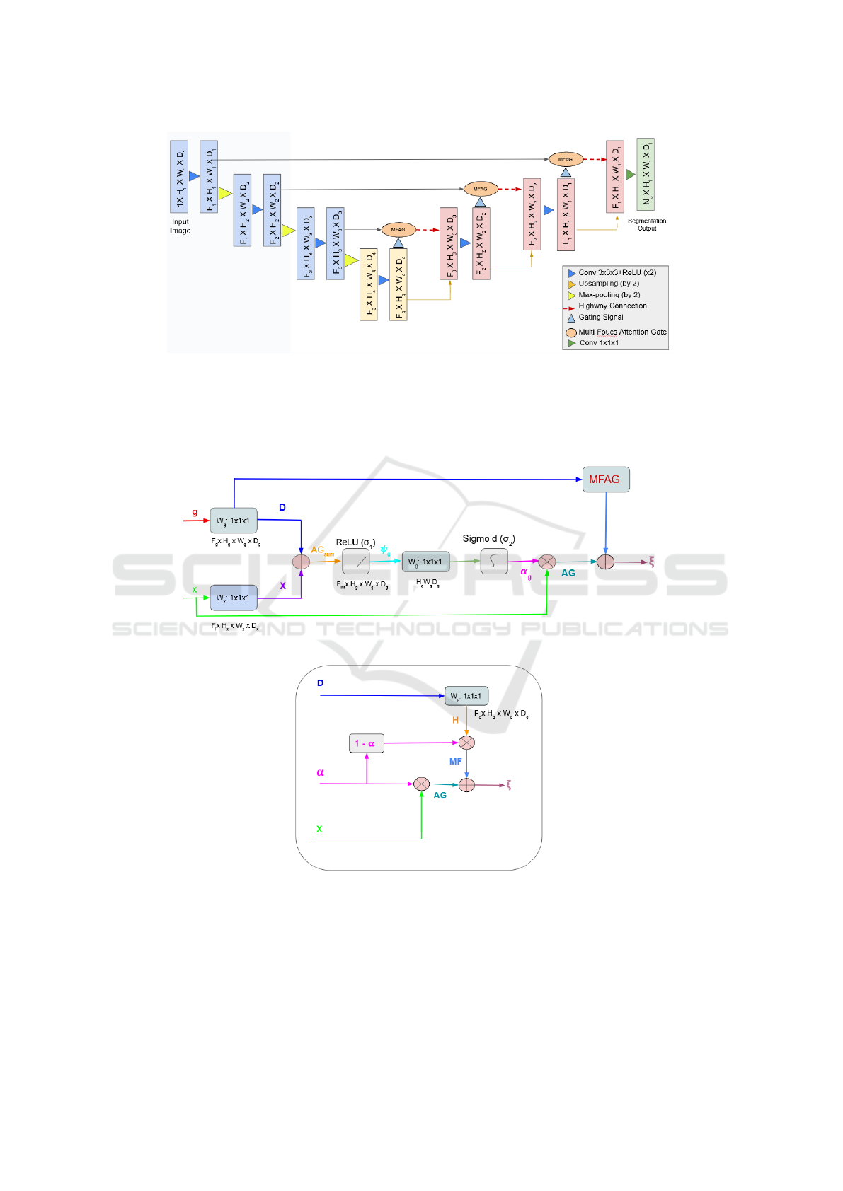
Figure 4: Block diagram of our proposed Multi-Focus Attention UNet (MFAU) model. The input image is downsampled in

the encoder path (blue) and upsampled in the decoder path (red). The bottleneck (yellow) is a bridge between the encoder

and decoder. Our model is similar to Attention UNet (Oktay et al., 2022); the differences lie in the features from the encoder

and decoder being passed through the MFAG (orange ellipses) and further through the highway skip-connections (red dashed

arrows). The ﬁnal layer is shown in green. The FxHxW xD represents the size of the feature maps where F is the number of

channels, and HxW xD are the height, width, and depth of the image. N

in the ﬁnal layer represents the number of instance

labels.

(a)

(b)

Figure 5: a) Block Diagram of the Multi-Focus Attention Gate. b) MFAG block. The attention coefﬁcient α, is computed

using the input feature (x) from the encoder and the gating signal (g) from the decoder. AG is the output of the attention gate.

The W

: 1x1x1 are 1x1x1 convolutions.

it for consistency. The following equation shows the

non-linear activation being applied:

= σ

(AG

sum

) = max(0, AG

sum

) (2)

where ψ

represents the intermediate coefﬁcients. A

linear transformation is applied to ψ using 1x1x1 con-

volutions (not using spatial dimensions), utilized to

downsample the input feature maps to the gating fea-

VISAPP 2024 - 19th International Conference on Computer Vision Theory and Applications

218

ture vector dimensions. A non-linear activation func-

tion, i.e., sigmoid (represented as σ

), is applied to

the linearly transformed results. We use a sigmoid

activation to yield sparser activations instead of a

softmax function that normalizes the attention coef-

ﬁcients, thus resulting in better training convergence

in Attention Gates (Oktay et al., 2022).

= σ

(ψ

) =

1 + e

−ψ

(3)

where α represents the attention coefﬁcients ∈ [0, 1],

which highlight feature responses from the salient re-

gions and suppress the ones with lesser semantic val-

ues. In AG, a grid resampler is applied to the attention

coefﬁcients that are implemented using trilinear inter-

polation to make the dimensions of the feature maps

similar to the dimensions of the input feature vector to

multiply them element-wise. In our case, the dimen-

sions of the attention coefﬁcient feature maps are the

same as the input feature vector x. Therefore, for the

purpose of simplicity, we omit this step. The element-

wise product of attention coefﬁcients with the input

feature vector from the encoding stage (i.e., used to

scale each spatial location of the input feature vector

based on the attention scores α ∈ [0, 1]), is given as:

= α

(4)

To perform the multi-focus attention mechanism

(see Figure 5b), the transformed gating feature vec-

tor, represented as D

, is sequentially transformed

again. This transformation serves the purpose of fur-

ther enhancing the gating features at a coarser scale

through the utilization of 1x1x1 convolution opera-

tions, denoted as H(g

) and parameterized by W

for multi-focus feature vectors (H(g

) is repre-

sented as H

for simplicity). This transformed gat-

ing feature vector is element-wise multiplied with the

complement of attention coefﬁcients to further im-

prove the focusing ability of the network, select the

most relevant features, and discard the less important

ones.

= (1 − α

).H

(5)

The ﬁnal output of the MFAG is given by concate-

nating Eqn. 4 with Eqn. 5:

= AG

+ MF

(6)

= α

+ (1 − α

).H

(7)

where ξ

represents the selection feature vectors at

layer l. The attention coefﬁcient α ∈ [0, 1] acts as

a weighting mechanism that controls the amount of

focus to be given to the input feature map from the

encoding stage or to the gating feature map from a

coarser decoding layer. If α is close to 0, the output of

the MFAG will focus more on the spatial information,

whereas if α is close to 1, the output will focus more

on the contextual information from the input image.

Based on the Eqn. 6, a special case of saturation

of the attention coefﬁcients α ∈ [0, 1] is given below:

(

x, if α = 0

H, if α = 1

(8)

For simplicity, the symbol for layer l has been

omitted. If α is 0, the input feature vectors from

the encoding stage are highlighted, whereas if α is

1, the gating feature vectors from the decoder layer

collected at a coarser scale undergo a linear transfor-

mation that helps to recognize complex patterns of the

feature map and highlight these patterns.

3.2 Highway Skip-Connections

There is plenty of evidence related to how the depth

of a neural network improves its performance; how-

ever, optimizing a deeper network is a challenging

task. Highway networks (Srivastava et al., 2015) were

explicitly designed to overcome these challenges and

train very deep neural networks. They introduce

adaptive gating units, a component that learns to con-

trol the ﬂow of information in the network. As a re-

sult, there can be paths through which the information

can traverse directly several layers without being al-

tered. These adaptive gating units (known as highway

connections) are used at each layer in the highway

networks and were inspired from the gating mecha-

nism used in Long-Short Term Memory (LSTM) net-

works (Graves and Graves, 2012). The main goal of

these gating functions is to learn to select whether

the information needs to be passed or transformed

through the network. This way, the network is able

to dynamically learn which features are relevant to a

particular problem and adapt accordingly. To the best

of our knowledge, we are the ﬁrst group to use the

concept of highway networks for a small number of

layers and integrate it with a UNet-based model as

skip-connections.

The output of the MFAG, represented as ξ

, acts as

an input to the highway connection at each decoding

layer l. Two sets of operations are applied on the input

feature vector ξ

: a transformation gate and a trans-

formation layer (the difference between these two op-

erations is the use of different non-linear activation

functions). These operations are deﬁned as G(ξ

)

and T (ξ

), parameterized by W

and W

at every

layer l for the transformation gate and transformed in-

put, respectively. The transformation gate consists of

a 1x1x1 convolution operation and a sigmoid func-

tion. This sigmoid function produces a value in the

Single-Class Instance Segmentation for Vectorization of Line Drawings

219

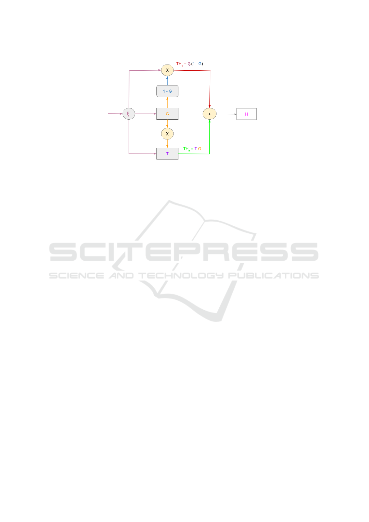
Figure 6: Block diagram of Highway Connections. ξ represents the input from the encoding stage, while H represents the

output of the Highway connections, G and T are the transformation gate and transformation layer, respectively. The red and

green path shows the two paths from where the information ﬂows.

range 0 and 1, depicting how much of the transformed

input should be passed through the networks. If the

value is close to 1, the input ﬂows through the layer,

whereas if the value is close to 0, most of the inputs

get transformed. The transformation layer consists of

a 1x1x1 convolution operation followed by a ReLU

function to apply a non-linear transformation on the

input image. The transformation function enables the

network to capture complex features from the input

image. The two non-linear activation functions are

used in a certain way to mitigate the vanishing gra-

dient problem, as even if the transformation gate col-

lapses due to saturation towards 0, the input is still

passed through the network. If the saturation of the

transformation gate approaches 1, the input gets fully

transformed (this special case is shown in Eqn. 13).

Information is passed through two neural paths

(the paths are shown in red and green in Figure 6).

In the ﬁrst path (red), the input feature vector ξ

is element-wise multiplied with the complement of

the transformation gate feature maps, represented as

1 − G(ξ

) (henceforth written as (1 - G)

for sim-

plicity). This element-wise product for the ﬁrst infor-

mation path is given as:

T H

= (1 − G)

.ξ

(9)

In the second information path (green), the feature

vectors from both the transformation gate G(ξ

)

(represented by G) and transformed input T (ξ

)

(represented by T) are element-wise multiplied by

each other at each layer l.

T H

= G

(10)

Highway connections are formed by combining

information paths constructed in Eqns. 9 and 10.

Therefore, the overall highway connections are rep-

resented as:

= T H

+ T H

(11)

= G

+ (1 − G)

.ξ

(12)

where H symbolizes highway connections output at

each decoding layer l. The dimensions of H, G, T and

ξ will always be the same.

Based on Eqn. 12, the special case of saturation of

the transformation gate can be given by the following

two conditions:

H =

(

ξ, if G = 0

T , if G = 1

(13)

For simplicity, the symbol for layer l has been

omitted. Therefore, depending on the value of the

transformation gate, highway connections control the

ﬂow of information by selecting whether to empha-

size the transformed input or the original input.

3.3 Compounded Loss Function

We have a speciﬁc use case that is inherently im-

balanced in a heavy-tailed distribution manner. The

output of the segmentation model consists of a static

number of channels, corresponding to the maximum

number of possible stroke instances (see Section 4.1).

As a result, we observe a dense distribution until the

average number of strokes followed by a decreasing

trend.

The output of the proposed instance segmentation

model is a static number of channels, which makes

this problem analogous to a multi-label classiﬁcation

problem. However, unlike a multi-label classiﬁca-

tion problem where each channel represents a speciﬁc

class prototype, in our use case, we do not have any

VISAPP 2024 - 19th International Conference on Computer Vision Theory and Applications

220

ﬁxed class prototype, i.e., any instance of the stroke

can appear in any channel. Moreover, different artists

have different drawing styles, as a result, the same

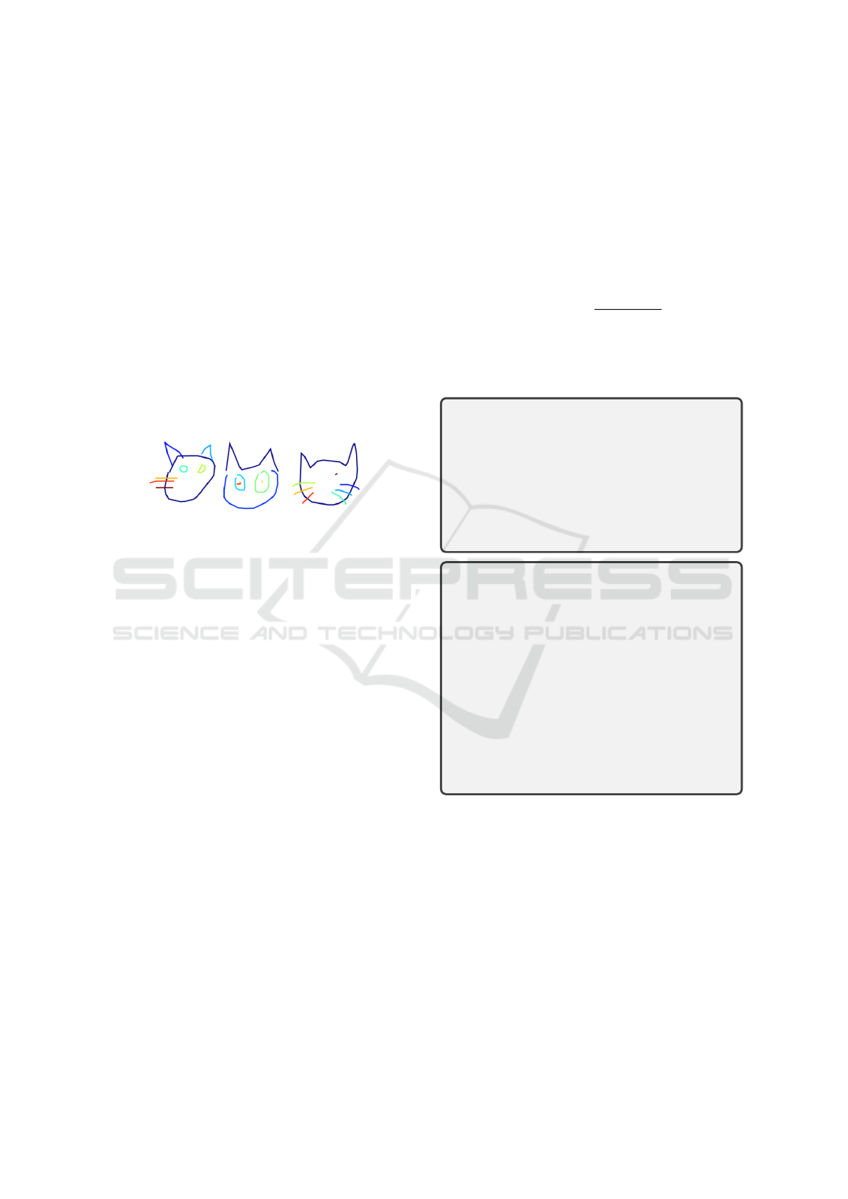
stroke can represent different instances. Figure 7 il-

lustrates different drawing styles for a cat; most of the

time a cat is drawn with two ears, a face, and each

whisker separately labeled, however, there are cases

where the two ears are labeled as a single entity, or

the whole face is labeled as one. The skewed distribu-

tion in our use case means that infrequent logit chan-

nels may suffer from ﬂoating point truncation. This

issue is mitigated by our margin scaling of the logits.

Margin scaling prevents dead neurons which allows

for the full power of the attention gates to be used to

model the pattern variability. Therefore, we propose

a loss function named Margin-Regularized Loss that

addresses this variation and identiﬁes the individual

instances accurately.

Figure 7: Example of variations of strokes in a cat dataset.

Left: The common way the cats are labeled. Middle: The

two ears are labeled as one and the face as another. Right:

The whole face is labeled as one.

Apart from assigning correct labels to each in-

stance of the stroke, we also need to consider the

spatial information of the strokes to incorporate the

precise positioning, overlapping, and relationship be-

tween these strokes. The spatial imbalances favor in-

stances with larger spatial strokes in the dataset to the

detriment of smaller ones. To address spatial imbal-

ance issues, Dice Loss is used to assess how well the

ground truth and predicted output overlap with each

other. It gives equal weights to pixel-wise true pos-

itives and false negatives, encouraging the model to

capture the spatial region correctly.

The total loss leverages the strength of both loss

components and is expressed as:

L = β ∗ DL(y

, y

) + (1 − β) ∗ S((y

, y

)) (14)

where β is a hyperparameter, DL(y

, y

) represents

the Dice Loss (Sorensen, 1948; Sudre et al., 2017) and

S((y

, y

)) represents the Margin-Regularised loss

(see Sec. 3.3.1). In our case, the value of β is 0.5

to equally leverage the beneﬁts of both the loss func-

tions.

3.3.1 Margin-Regularized Loss Function

Inspired by Label-Distribution-Aware Margin

(LDAM) (Cao et al., 2019), we developed a loss

function that calculates the loss in three steps: (1)

calculating the margins, (2) margin scaling, and (3)

adding a regularization term.

Let y

and y

represent the ground truth la-

bels and predicted outputs. The predicted output

of the model for N classes can be written as z

, z

, ...., z

]

. The i

output of the model f can

be deﬁned as z

= f (y

)

. The margins are calculated

in the following way (similar to a sigmoid function):

M(y

, y

) =

1 + se

−y

(15a)

0 ≤ M(x, y) ≤ 1 (15b)

where s is a scaling factor. The value of s, in our case,

is 200 and has been experimentally determined.

Observation 1. (Asymptotic Behaviour)

As xy → ∞, M(x, y) → 1 when s > 0 and

M(x, y) → 0 when s < 0

Proof. If lim

xy→∞

M(x, y), then e

−xy

→ 0, and,

if s > 0, se

−xy

→ 0. As a result, (1+se

−xy

) →

1 and M(x, y) → 1. Conversely, if s < 0, se

−xy

still approaches 0. However, (1 + se

−xy

) → 0

and M(x, y) → 0.

Observation 2. Due to the randomness of the

labels in the training data, the margin M(x, y)

is bounded between 0 and 1 for all the real

values of x and y.

Proof. As we know, the value of e

−xy

lies

between 0 and 1, i.e., it will always be pos-

itive for all the real values of x and y. There-

fore, the denominator 1 + se

−xy

will always

be positive and is bounded between 0 and

s+1. When the denominator is inversed, the

bounded range is back to the interval (0, 1).

As a result, M(x, y) is always bounded by 0

and 1.

Eqn. 15a is used to scale margins and apply enforced

margins in a cross-entropy loss function. The scaling

of the margins is performed as follows:

∆

= (1 − M(y

, y

)).y

+ M(y

, y

).y

(16)

where ∆

represents the margin scaling term. The

cross-entropy loss function with enforced margins is

given below:

CE(y

, y

) = −

∑

j=1

. log ∆

(17)

In order to avoid overﬁtting and improve feature

selection by encouraging the sparser set of feature

Single-Class Instance Segmentation for Vectorization of Line Drawings

221

weights, the L1 regularization term (i.e., the summa-

tion of the absolute values of the model’s coefﬁcient)

is added to the above loss function. In our initial

study, we tested our loss function for both L1 and L2

regularization terms and found that our training model

converges better with L1 regularization. As a result,

we use the L1 regularization:

S(y

, y

) = CE(y

, y

) + λ

∑

| (18)

where λ is a hyperparameter that controls the amount

of regularization.

4 EXPERIMENTAL EVALUATION

The performance of our proposed model is assessed

and compared against the state of the art (Kim et al.,

2018), as well as against the Attention UNet (Ok-

tay et al., 2022), a model which we have built upon.

Section 4.1 provides information about the datasets,

and the construction of labeled ground truth. Sec-

tion 4.2 discusses implementation details and also ex-

plains how we constructed our ground truth and how

we vectorized the output of our proposed approach.

Sections 4.3 and 4.4 analyze the performance of our

method in both quantitative and qualitative ways.

4.1 Datasets

We evaluate our model on six datasets constructed by

(Kim et al., 2018). They belong to three semantically

distinct categories: characters (Chinese and Kanji),

synthetic random lines (Lines), and sketches (Base-

ball, Cat, and Multi-Class). Each dataset consists of

images in SVG format which are divided into training

and testing sets; the distribution is described in Ta-

ble 1. To prevent overﬁtting and improve the model’s

ability to generalize on unseen data, we created a val-

idation set by further splitting the training set into a

70:30 ratio. Additionally, we are dealing with a spe-

ciﬁc use case that is inherently imbalanced in a heavy-

tailed distribution manner. When evaluating the over-

all performance of each dataset, it is important to con-

sider the distribution of the number of strokes within

the dataset. Table 2 gives details about the number of

vector paths used in each dataset.

The datasets from (Kim et al., 2018) are in SVG

format. To use these data for training purposes, we

need to convert them back to raster: the CairoSVG

library is used to convert SVG to PNG, outputting

(https://pypi.org/project/CairoSVG/)

Table 1: The number of images used for training, validation,

and testing purposes.

Chinese Kanji Line Baseball Cat Multi

Train 5989 7216 31499 85285 77616 56000

Val 2567 3093 13500 36551 33264 24000

Test 951 1145 4999 13536 12318 8888

grayscale input raster images that are used for train-

ing. To generate the ground truth, each path extracted

from the vector image is individually processed, cre-

ating a binary representation where all pixels within a

path receive the same label. These labeled masks are

then combined to form the ﬁnal ground truth image.

When assigning labels to each pixel along the path,

pixels belonging to overlapping regions will ideally

be assigned multiple labels. We opt for a simpler la-

belling approach and assign each pixel in the overlap

the label of the last path passing through it. This ap-

proach ensures a coherent labeling strategy while en-

abling us to still detect strokes with some minor dis-

continuities.

4.2 Implementation

Our PyTorch model was trained on a GPU cluster with

four NVIDIA P100 GPU with 12 GB of memory. The

inference was performed separately on a single desk-

top NVIDIA GeForce GTX 1660 Ti GPU with 6 GB

of memory so that an accurate runtime measurement

could be obtained. For the characters and random line

datasets, we trained our model for 500 epochs with

an image size of 64 × 64 and batch size of 8. For

the sketch datasets, we used a batch size of 32 and an

image size of 128 × 128 and trained for 200 epochs.

We trained our model using the Adam optimizer

(Kingma and Ba, 2017) and an initial learning rate of

−4

. The maximum number of labels used for train-

ing our model is ﬁxed at 128. Although this number

is signiﬁcantly larger than the highest number of vec-

tor paths among all the six datasets, it was chosen to

maintain consistency with (Kim et al., 2018). Also,

opting for this value did not have any negative impact

on our model’s performance. The scaling factor used

in our loss function is 200, and the weight used for the

compounded loss function is 0.5. These values were

determined experimentally during the hyperparame-

ter optimization of the datasets.

4.3 Quantitative Analysis

To evaluate our results, we measure per-stroke

intersection-over-union (IoU) between our ﬁnal out-

put and its corresponding ground truth. Our results

are compiled and compared to reference methods in

Table 3. Overall, our method performed well for

VISAPP 2024 - 19th International Conference on Computer Vision Theory and Applications

222

Table 2: The minimum, maximum, mode, mean and standard deviation of the number of vector paths (i.e., stroke instances)

used in training/validation and testing phase for each dataset.

Dataset Minimum Maximum Mode Mean Std

Train Test Train Test Train Test Train Test Train Test

Chinese 1 1 33 28 11 10 11.75 11.73 4.39 4.32

Kanji 1 1 30 29 12 12 12.58 12.39 4.79 4.76

Random 4 4 4 4 4 4 4 4 0 0

Baseball 1 1 84 55 3 3 4.98 4.98 3.34 3.34

Cat 1 1 40 31 9 9 9.87 9.85 3.88 3.90

Multi-Class 1 1 115 48 3 3 7.03 7.0 4.50 4.45

Table 3: Per-pixel intersection-over-union (IoU) performed on the test set. Best results are shown in bold font. The IoU

average excludes the random lines dataset, which was included as a counter-example.

Chinese Kanji Baseball Cat Multi-Class Avg. Random

(Kim et al., 2018) 0.958 0.917 0.827 0.811 0.753 0.853 0.872

Attention UNet 0.884 0.918 0.853 0.433 0.742 0.766 0.276

Ours 0.937 0.946 0.869 0.831 0.786 0.874 0.271

Table 4: Average execution time taken by a single image at inference (in seconds).

Chinese Kanji Random Baseball Cat Multi-Class

(Kim et al., 2018) 54.9 26.589 8.46 853 233 409

Attention UNet 0.0106 0.0154 0.0146 0.0404 0.0365 0.0389

Ours 0.0089 0.0095 0.0231 0.0179 0.0223 0.0109

Table 5: Computational Complexity, measured in terms of

number of parameters and GFLOPS. The down arrow indi-

cates that it is better to have low values.

Model Number of Parameters ↓ GFLOPs ↓

(Kim et al., 2018) 1.34 M 0.00266

Attention UNet 34.9 M 4.19

Ours 32.8 M 3.79

most of the datasets in terms of accuracy. However,

for Chinese characters, (Kim et al., 2018) performed

slightly better (+0.012) than our model. Our method

requires a larger amount of data for increased perfor-

mance; the Chinese dataset contains the least num-

ber of training images. However, we outperformed

the other methods on the other datasets (excluding the

random line dataset). This points towards our model’s

ability to generalize effectively when provided with a

large dataset.

The outlier in performance is the random line

dataset; our method outperformed (Kim et al., 2018)

by an average of 0.0208 when excluding the random

lines dataset. The IoU for the random line dataset

for both Attention UNet and our method is less than

0.30, despite this dataset consisting of only four la-

bels. This poor performance can be attributed to the

totally random nature of the strokes, containing no

spatial relationship between them. We hypothesize

that as our model captures spatial relationships well,

in the absence of these relationships, we are essen-

tially training on “noise”. Therefore, this serves as

a counter-example, demonstrating our model’s abil-

ity to leverage the spatial relationships between the

instances, as it is able to perform well on all other

datasets with more semantically structured contents.

4.3.1 Computation Time

We have compared the average computation time

taken per image at the inference of our proposed

model with the (Kim et al., 2018) method and Atten-

tion UNet. As shown in Table 4, our approach takes

less than 50 milliseconds and is 1711500% and 64%

faster than the (Kim et al., 2018) method and the At-

tention UNet, respectively.

4.3.2 Computation Complexity

The computation complexity, in terms of GFLOPs,

and the number of parameters of our model and com-

parable approaches is shown in Table 5. Despite be-

ing less complex and having fewer parameters, (Kim

et al., 2018) requires a signiﬁcantly higher execu-

tion time. However, the calculation of the number of

model parameters and GFLOPs does not include the

iterative optimization of the Markov Random Field

(MRF); as a result, the parameters and the ﬂoating

Single-Class Instance Segmentation for Vectorization of Line Drawings

223

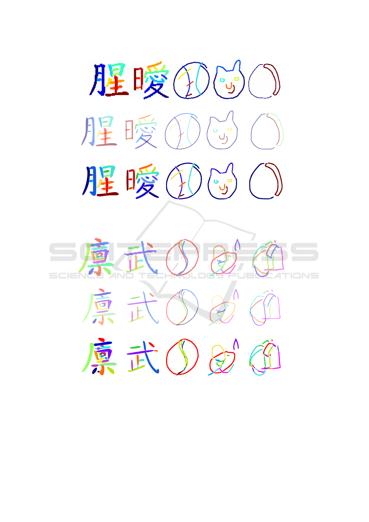
(a) Chinese (b) Kanji (c) Baseball (d) Cat (e) (Multi)

(f) 0.97 (g) 0.94 (h) 0.78 (i) 0.78 (j) 0.67

(k) 0.99 (l) 0.99 (m) 0.98 (n) 0.83 (o) 0.99

Figure 8: Stroke-based Comparison between (Kim et al., 2018) and Our Method on Chinese, Kanji, Baseball, Cat and Multi-

Class dataset for successful cases, where First row: Ground truth, Middle row: Kim et al. IoU results Last row: Our IoU

results.

(a) Chinese (b) Kanji (c) Baseball (d) Cat

(e) Backpack (Multi)

(f) 0.97 (g) 0.94 (h) 0.78 (i) 0.78 (j) 0.67

(k) 0.83 (l) 0.92 (m) 0.55 (n) 0.73 (o) 0.39

Figure 9: Stroke-based Comparison between (Kim et al., 2018) and Our Method on Chinese, Kanji, Baseball, Cat and Multi-

Class dataset for successful cases, where First row: Ground truth, Middle row: Kim et al. IoU results. Last row: Our IoU

results.

point operations calculated are signiﬁcantly less than

ours. Hence, comparing our model with (Kim et al.,

2018) based on the computation complexity of the

model may not be relevant.

Our proposed model demonstrates superiority

over Attention UNet in terms of both model parame-

ters and model complexity. Attention UNet has more

than 2.1 million additional parameters compared to

VISAPP 2024 - 19th International Conference on Computer Vision Theory and Applications

224

our proposed approach. Additionally, in terms of

GFLOPs, our model showcases a reduction of 0.4

compared to the Attention UNet. This highlights our

model’s efﬁciency in terms of both parameter count

and computational workload.

4.4 Qualitative Analysis

We visually compare our outputs with those of (Kim

et al., 2018) using examples from all datasets except

the random lines. Although both methods are able

to segment correct instances of strokes in most cases,

both have distinct shortcomings.

Figure 8 presents examples where our method per-

formed qualitatively better than (Kim et al., 2018). As

shown in Figure 8k and Figure 8l, despite the pres-

ence of a missing pixel in the overlapping regions of

the ground truth, we are still able to maintain conti-

nuity in the strokes. A user can draw a cat in various

styles, such as using a single stroke for the whole face,

two separate strokes for the ears and face, or individ-

ual strokes for the ears and face. In Figure 8n, our

model not only segments the instances but also infers

the user’s drawing style. This stands in contrast to

(Kim et al., 2018), as shown in Figure 8i, which erro-

neously predicts the face and ears as one stroke (i.e.

the most common drawing style).

Figure 9 shows some shortcomings of our method

when compared to (Kim et al., 2018). In the char-

acter dataset (shown in Figure 9k and Figure 9l), it

can be observed that multiple instances are assigned

to a single stroke instance, resulting in a phenomenon

known as “vector soup”. However, if human interven-

tion is allowed as a postprocessing step, the number

of required edits would be minimal; thus our output

could be successfully utilized for further editing. In

Figure 9m and Figure 9n, some of the instances were

mislabeled, however, our model accurately identiﬁes

circles in both categories, unlike (Kim et al., 2018).

Overall, it can be concluded that our model is able

to follow three main perceptual grouping principles

(similarity, continuity and closure).

5 CONCLUSIONS

We propose a novel segmentation method that pro-

cesses the input raster image by labeling each pixel as

belonging to a particular stroke instance. Our novel

architecture, named Multi-Focus Attention UNet

builds upon Attention UNet by introducing multi-

focus attention gates and highway skip connections,

two architectural elements which play a key role in

capturing global and local image context and in high

computational efﬁciency. Our loss function includes

a margin-regularised component which allows us to

handle successfully a heavy-tailed label distribution,

as well as infer correctly the user’s drawing style. Our

approach is signiﬁcantly faster, exceeding state of the

art by seven orders of magnitudes. Future work in-

volves extending our focus to complex line drawing

art that would signiﬁcantly beneﬁt from image vec-

torization when shown on large displays.

REFERENCES

Bartolo, A., Camilleri, K. P., Fabri, S. G., Borg, J. C., and

Farrugia, P. J. (2007). Scribbles to vectors: prepa-

ration of scribble drawings for cad interpretation. In

Proceedings of the 4th Eurographics workshop on

Sketch-based interfaces and modeling, pages 123–

130.

Bouton, G. D. (2014). CorelDRAW X7. Mcgraw-hill

Education-Europe.

Cao, K., Wei, C., Gaidon, A., Arechiga, N., and Ma, T.

(2019). Learning imbalanced datasets with label-

distribution-aware margin loss. Advances in neural

information processing systems, 32.

de Casteljau, P. (1963). “courbes et surfaces a poles,” tech-

nical report. Citroen, Paris.

Dori, D. (1997). Orthogonal zig-zag: an algorithm

for vectorizing engineering drawings compared with

hough transform. Advances in Engineering Software,

28(1):11–24.

Favreau, J.-D., Lafarge, F., and Bousseau, A. (2016). Fi-

delity vs. simplicity: a global approach to line drawing

vectorization. ACM Transactions on Graphics (TOG),

35(4):1–10.

Graves, A. and Graves, A. (2012). Long short-term mem-

ory. Supervised sequence labelling with recurrent

neural networks, pages 37–45.

He, K., Gkioxari, G., Dollar, P., and Girshick, R. (2017).

Mask r-cnn. In Proceedings of the IEEE ICCV.

Hilaire, X. and Tombre, K. (2006). Robust and accu-

rate vectorization of line drawings. IEEE Transac-

tions on Pattern Analysis and Machine Intelligence,

28(6):890–904.

Inoue, N. and Yamasaki, T. (2019). Fast instance seg-

mentation for line drawing vectorization. In 2019

IEEE Fifth International Conference on Multimedia

Big Data (BigMM), pages 262–265. IEEE.

Jimenez, J. and Navalon, J. L. (1982). Some experiments

in image vectorization. IBM Journal of research and

Development, 26(6):724–734.

Kim, B., Wang, O.,

Oztireli, A. C., and Gross, M. (2018).

Semantic segmentation for line drawing vectorization

using neural networks. In Computer Graphics Forum,

volume 37, pages 329–338. Wiley Online Library.

Kingma, D. P. and Ba, J. (2017). Adam: A method for

stochastic optimization.

Single-Class Instance Segmentation for Vectorization of Line Drawings

225

Kultanen, P. (1990). Randomized hough transform (rht)

in engineering drawing vectorization system. Proc.

MVA, pages 173–176.

Najgebauer, P. and Scherer, R. (2019). Inertia-based fast

vectorization of line drawings. In Computer Graph-

ics Forum, volume 38, pages 203–213. Wiley Online

Library.

Oktay, O., Schlemper, J., Le Folgoc, L., Lee, M., Heinrich,

M., Misawa, K., Mori, K., McDonagh, S., Hammerla,

N. Y., Kainz, B., et al. (2022). Attention u-net: Learn-

ing where to look for the pancreas. In Medical Imag-

ing with Deep Learning.

Roosli, M. and Monagan, G. (1996). Adding geomet-

ric constraints to the vectorization of line drawings.

In Graphics Recognition Methods and Applications:

First International Workshop, pages 49–56. Springer.

Selinger, P. (2003). Potrace: a polygon-based tracing algo-

rithm.

Sorensen, T. A. (1948). A method of establishing groups of

equal amplitude in plant sociology based on similarity

of species content and its application to analyses of the

vegetation on danish commons. Biol. Skar., 5:1–34.

Srivastava, R. K., Greff, K., and Schmidhuber, J. (2015).

Training very deep networks. Advances in neural in-

formation processing systems, 28.

Sudre, C. H., Li, W., Vercauteren, T., Ourselin, S., and

Jorge Cardoso, M. (2017). Generalised dice overlap

as a deep learning loss function for highly unbalanced

segmentations. In Deep Learning in Medical Image

Analysis and Multimodal Learning for Clinical De-

cision Support: Third International Workshop, pages

240–248. Springer.

Tombre, K., Ah-Soon, C., Dosch, P., Masini, G., and Tab-

bone, S. (2000). Stable and robust vectorization: How

to make the right choices. In Graphics Recogni-

tion Recent Advances: Third International Workshop,

pages 3–18. Springer.

Wood, B. (2012). Adobe illustrator CS6 classroom in a

book. Adobe Press.

Zhang, Y., Zhu, M., Zhang, Q., Shen, T., and Zhang, B.

(2022). An approach of line vectorization of engi-

neering drawings based on semantic segmentation. In

2022 IEEE 17th Conference on ICIEA, pages 1447–

1453. IEEE.

VISAPP 2024 - 19th International Conference on Computer Vision Theory and Applications

226