Swap-Deep Neural Network: Incremental Inference and Learning for

Embedded Systems

Taihei Asai and Koichiro Yamauchi

Institute of Computer Science, Chubu University, Matsumoto-cho 1200, Kasugai, Aichi, Japan

Keywords:

Hidden Neural Network, Incremental Learning, Continual Learning, Deep Neural Networks.

Abstract:

We propose a new architecture called “swap-deep neural network” that enables the learning and inference

of large-scale artiﬁcial neural networks on edge devices with low power consumption and computational

complexity. The proposed method is based on ﬁnding and integrating subnetworks from randomly initial-

ized networks for each incremental learning phase. We demonstrate that our method achieves a performance

equivalent to that of conventional deep neural networks for a variety of various classiﬁcation tasks.

1 INTRODUCTION

One reason for the rapid development of artiﬁcial in-

telligence in recent years is the establishment of learn-

ing methods for large-scale neural networks. In sev-

eral cases, the neural network connections that are es-

sential for realizing a complex task do not need to

be considerably large. However, large-scale neural

networks are typically required to achieve success-

ful learning. This is because the probability of the

initial state of the connections required for the task

to be included in the randomly initialized neural net-

work does not increase unless the scale is large. In

other words, to successfully achieve both learning and

recognition, it is desirable for the neural network to be

as large as possible.

However, to practically realize such learning and

inference, it is necessary to implement them on edge

devices. Many existing edge devices are connected

to cloud servers via the Internet and their heavy com-

putational tasks are performed by the cloud servers.

Particularly, they request the cloud server to perform

the learning process and transfer back the resulting

weight parameters. However, this system faces the

risk of privacy leakage associated with network con-

nections.

One way to solve this problem is to compress the

large neural network to a small one. For example,

some methods are the neural architecture selection

(NAS) (e.g. (Sadel et al., 2023)), pruning useless con-

nections by using the regularization term(Ishikawa,

https://orcid.org/0000-0003-1477-0391

1996) and distillation techniques(Hinton et al., 2015).

These methods require all required samples to be pre-

pared in advance. Moreover, in the case of the NAS,

the system has to prepare several solution-candidates

to ﬁnd a better solution. These conditions are too

hard to manage the system on-site, where the system

has to incrementally learn new novel samples with a

bounded memory space.

In this study, we propose a novel method to solve

this problem. In particular, we propose a method for

realizing both learning and inference on edge devices

without connecting them to cloud servers. However,

we assume a situation in which the size of the neural

network required to learn and recognize a task that the

user faces exceeds the capacity of the edge device. In

this case, the proposed method divides the task into

multiple subtasks and trains each subtask on a sepa-

rate network on the edge device. The parameters real-

ized in this manner are stored on a secondary storage

device; during inference, the parameters are read in

sequence and inferred, and the results are ensembled.

However, this increases the power consumption ow-

ing to data transfer. Therefore, we infer subtasks in

a manner similar to that of a hidden neural network

(Ramanujan et al., 2020), using randomly initialized

neural networks. In other words, we identify and re-

tain only a few important weight connections that are

necessary for inferring the subtask and store their po-

sition information on a secondary storage device. We

expect that the power and time consumed during read-

ing will be reduced.

In this paper, we present the theoretical analysis of

power consumption and a simulation result. The re-

418

Asai, T. and Yamauchi, K.

Swap-Deep Neural Network: Incremental Inference and Learning for Embedded Systems.

DOI: 10.5220/0012465500003654

Paper published under CC license (CC BY-NC-ND 4.0)

In Proceedings of the 13th International Conference on Pattern Recognition Applications and Methods (ICPRAM 2024), pages 418-427

ISBN: 978-989-758-684-2; ISSN: 2184-4313

mainder of this paper is organized as follows. Section

2 describes related work. Section 3 presents a review

of hidden neural networks. Section 4 describes the

proposed incremental learning method. Section 5 an-

alyze the power-consumption of the proposed learn-

ing method. Section 6 presents the experimental re-

sults and Section 7 discusses the computational com-

plexity and suitable learning strategy of the proposed

system. Finally Section 8 concludes the paper.

2 RELATED WORKS

The learning of dividing a task into multiple subtasks

and learning them individually can be considered in-

cremental learning (continual learning). At the same

time, this method of learning a task as multiple sub-

tasks and integrating them is also known as ensemble

learning, particularly boosting method. Furthermore,

there are several techniques for reducing power con-

sumption and increasing processing efﬁciency when

implemented on edge devices. In this section, we

compare the differences between existing methods

and the proposed method.

2.1 Comparison with Boosting Methods

A classical boosting method, Adaboost (Freund and

Schapire, 1997), ﬁxes weights by learning with weak

learners. A weak learner increases the weight of the

incorrect learning sample, decreases the weight of the

correct learning sample, and then learns with the next

weak learner. Using the set of weak learners created

in this manner, unknown inputs are inferred in par-

allel. The average of the answers obtained in this

manner is weighted and the ﬁnal output is obtained,

resulting in a higher recognition rate than that of indi-

vidual weak learners. This method is not suitable for

learning in a completely divided data form as done in

the proposed method, because it uses the same dataset

for all subnetworks (weak learners). In contrast, Fos-

ter (Feature boosting) (Wang et al., 2022) assumes

that different domain learning samples are added to

learn instead of the same domain learning samples as

Adaboost. Therefore, this method is similar to the

proposed method and we incorporate Foster’s concept

into the proposed method. However, Foster adopted a

form of parallel computation that maintained the pa-

rameters of each subnetwork, which was not suitable

for low-power computation on edge devices, as as-

sumed in the proposed method.

In our method, we adopt a method of apply the

connection position information used in each subnet-

work to a network initialized randomly in each sub-

network by incorporating a hidden neural network

(Ramanujan et al., 2020) method, which is suitable

for cases in which all subnetworks share and use small

edge-device resources.

2.2 Comparison with Existing

Incremental Learning Methods

When new domain data are learned using an exist-

ing neural network, Catastrophic Forgetting (French,

1999) occurs. There are two main methods to prevent

this problem. One is to learn new domain samples to-

gether with old domain samples (e.g. (French, 1997),

(Yamauchi et al., 1999), (Hsu et al., 2018), (Hayes

et al., 2019)). These methods have the advantage that

once learned, past memories are not only prevented

from catastrophic forgetting but also reset by relearn-

ing. Our proposed method adopts a similar approach

in that it uses past data to set the parameters. How-

ever, networks that have been learned in the past by

ﬁxing their parameters are not relearned. The advan-

tage of this method is that it reduces the number of

computations required. The second method is to ﬁx

few weight parameters ((Rusu et al., 2016), (Kirk-

patrick et al., 2017) (Zenke et al., 2017) (Mallya and

Lazebnik, 2018) (Wang et al., 2022)) to ensure that

what has been learned in the past is preserved. Our

proposed method is similar to these methods in that

it ﬁxes the parameters learned in the past. However,

in principle, only the model proposed by Wang et al.

(Wang et al., 2022) can sequentially load and calcu-

late these ﬁxed parameters in order and calculate the

ﬁnal output. However, as mentioned previously, no

model among them considers the implementation on

edge devices.

2.3 Comparison with Neuromorphic

Computing

Neuromorphic computing is a general term for mod-

els that can efﬁciently compute neural networks by

providing hardware specialized for neural network

computation (Zheng and Mazumder, 2020). In con-

trast, the proposed method does not use a neuromor-

phic model. This is merely a proposal on operating

hardware with limited computing resources. How-

ever, more efﬁcient operations can be achieved by

executing individual neural networks in the neuro-

morphic models. Hirose et al. (Hirose et al., 2022)

proposed a novel hardware neural network that re-

duced power consumption by introducing a hidden

neural network architecture (Ramanujan et al., 2020).

We also introduce the same aspects as (Hirose et al.,

2022) to reduce power consumption. The difference

Swap-Deep Neural Network: Incremental Inference and Learning for Embedded Systems

419

between the proposed method and the model pro-

posed by (Hirose et al., 2022) is that the proposed

method supports incremental learning in large- scale

tasks.

2.4 Contribution of Our Proposed

Method

Our method virtually realizes a large-scale neural net-

work on hardware with limited computing resources,

while inheriting the ideas of the abovementioned ex-

isting methods. The differences between our method

and other methods are summarized in Table 1.

3 REVIEW OF HIDDEN NEURAL

NETWORK

Before describing the proposed method, this section

reviews the hidden neural network used in the pro-

posed method, as explained in Section . Ramanujan

et al. (Ramanujan et al., 2020) found that randomly

initialized neural networks include a subnetwork suit-

able for solving a speciﬁed task. They also presented

an effective method for ﬁnding a subnetwork using a

gradient descent method. Although this network uses

the gradient descent method, it does not modify the

weight parameters but ﬁnds the subnetwork.

3.1 Subnetwork

The subnetwork of a fully connected neural network

is described as follows (Ramanujan et al., 2020). The

l-th layer of a fully connected neuron consists of n

nodes V

(l)

= {v

(l)

,··· ,v

(l)

}. The subnetwork

found via gradient descent is described by G(V , E).

The node v ∈ V output is denoted as

= σ(I

) (1)

where σ() is the ReLU (Krizhevsky et al., 2012) and

is given as

∑

(u,v)∈E

(2)

To ﬁnd a good sub-network, a score s

for each

weight is introduced. The top k-percent of the ab-

solute values of the scores are selected as the subnet-

work. Therefore, (2) can be written as

∑

u∈V

(l−1)

h(s

), (3)

where h(s

) = 1 if |s

| is included in the top k

scores. In the case of the convolution layer, the scor-

ing method is almost the same as that of the fully con-

nected layer, except that the nodes are replaced with

channels.

3.2 Find a Good Sub-Network

(EDGE-POPUP)

Although the weight parameter values are ﬁxed at ran-

dom values, the score values s

are optimized using

a gradient descent algorithm as follows:

= s

−η

∂L

∂s

, (4)

where L denotes the loss function. Note that we have

to rewrite (3) to

∑

u∈V

(l−1)

| (5)

to calculate the gradient in (4)

The above equation omits the momentum and

weight decay terms. Moreover, the change in the

learning rate η is also ignored. These omitted terms

should be added according to the optimization method

used.

4 SWAP-DEEP NEURAL

NETWORK

The proposed learning system:Swap-deep neural net-

work (Swap-NN) consists of two parts: a convectional

neural network (CNN) and a secondary-storage (see

Fig 1). The CNN parameters are randomly initialized

and ﬁxed. Instead, CNN adaptation is achieved by

identifying the important connections found using (2)

and (4). The indices of the top k-scored connections

are stored in the secondary-storage.

We assume that the proposed learning system is

suitable for classiﬁcation tasks. Learning samples are

divided into several groups based on their labels. For

example, consider the case of dividing the MNIST

dataset into two groups. To realize this, the sam-

ples are divided for every ﬁve labels: {0,1,2,3,4},

{5,6,7,8,9}. In this case, the learning system gener-

ates two subnetworks to learn the datasets. Therefore,

The ’simple minist example’ presented by the authors

https://github.com/allenai/hidden-networks/ , L is cal-

culated by using (3). However, the backward calculation

for the L is executed by (5). This means that the learning

method is slightly different from (4). However, we found

that the convergence speed of the simple sample code is

faster than the code which derives L by (5). So, we have

developed our code based on the ’simple mnist example’.

ICPRAM 2024 - 13th International Conference on Pattern Recognition Applications and Methods

420

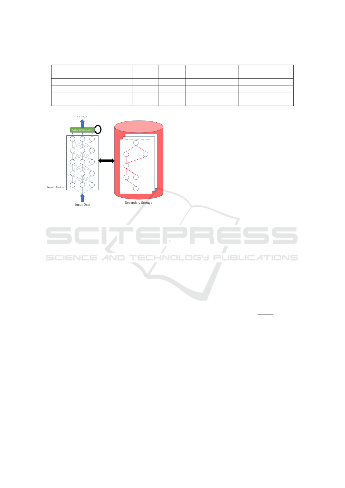
Table 1: Comparison with the other similar methods.

SwapNN

(ours)

Foster Feature

boost

Hidden

ıve re-

hearsal

PackNet

Learning of large-scale dataset ⃝ ⃝ ⃝ ⃝ ⃝ ⃝

Incremental Learning ⃝ ⃝ × × ⃝ ⃝

Execution on a small device ⃝ × × ⃝ × ×

Low-power consumption ⃝ × × ⃝ × ×

Figure 1: System structure: CNN with aggregation

layer(left), and secondary storage(right).

the ﬁrst subetwork learns the dataset whose labels are

{0,1,2,3,4} using (4). After learning, the most im-

portant k-connection indices and corressponding full-

connection(FC) layer parameters are stored in the sec-

ondary storage. Similarly, the second subnetwork

learns the datasets which have labels of {5,6,7,8,9}

together with a part of the ﬁrst dataset, in the same

manner as the ﬁrst subnetwork, and stores a k impor-

tant connection index and FC layer parameter. Dur-

ing the inference phase, an unknown input is assigned

to the input layer of the CNN. The system loads the

ﬁrst subnetwork connection indices and FC-layer pa-

rameters from the secondary storage and calculates

them. The output is sent to the aggregation layer,

which consists of the FC layers used by Foster (Wang

et al., 2022). The FC layers are also adjusted for opti-

mal mixing of all subnetwork outputs. This algorithm

is explained in Section 4.2. The second subnetwork

connection information is also loaded from the sec-

ondary storage, and CNN output is calculated. The

output is sent to the FC layers and the two sets of

outputs are aggregated (see Fig 2). The aggregated

output is the ﬁnal output of the system. Therefore, the

proposed network executes inferences sequentially by

swapping the current connection with next subnet-

work connection one by one (see Algorithm 2).

4.1 Problem Formulation

We assume that incremental learning is performed

when a novel sample set is presented. Let χ

≡

{(x

(t)

)}

p=1

be the novel sample set at t, where

t = 1,2,··· ,T . The learning system learns χ

at the t-

th incremental learning phase by referring old sample

sets stored in χ

old

, where |χ

old

| ≤ B. The old sam-

ples are needed for the learner to obtain better class-

boundaries. To store current data into |χ

old

|, an ele-

ment in χ

old

is randomly selected to be disposed such

that the condition |χ

old

| ≤ B holds (see Algorithm 1).

After each incremental learning phase, the learn-

ing system is evaluated by using test datasets,

which include all classes included in χ

, where t =

1,2,··· ,T . To prevent catastrophic forgetting, the

past scores s

at t = 1, ··· ,t −1 are not modiﬁed dur-

ing the later learning phases.

4.2 Incremental Learning by Adding

Sub-Networks

During the t-th incremental learning phase, the t-th

sub-network S

(t)

learns (x

(t)

) ∈ χ

∪ χ

old

from

scratch. Let ∆s

(t)

be the change in the score for w

∆s

(t)

derived by the steepest gradient descent with a

momentum term. Therefore,

∆s

(t)

= 0.9∆s

(t−1)

−η

∂L

∂s

(t−1)

, (6)

where L denotes the cross-entropy loss, s

(t)

denotes

the score of the w

at t, η denotes the learning speed

and η < 1. s

(t)

is modiﬁed as

(t)

= s

(t−1)

+ ∆s

(t)

. (7)

Note that the learning of samples in χ

∪χ

old

makes

the sub-network acquire correct classiﬁcation bound-

aries between the target class and the other classes.

After learning, the fully-connected aggregation layer

in the subnetwork is stored as the connection set for

the k maximum scores.

= {(u,v)|h(s

(t)

) = 1}, (8)

Swap-Deep Neural Network: Incremental Inference and Learning for Embedded Systems

421

where the function h(·) is the same function used in

(3). The summarized algorithm is shown in 1. After

the learning S

is stored in the 2nd storage.

Data: χ

,χ

old

Result: S

,χ

old

Initialize s

(0)

for i = 1 to NumE poch do

for (x,y) in χ

∪χ

old

Calculate L by using S

Score Update by (6), (7).

end

= {(u,v)|h(s

(t)

) = 1}

for i = 1 to NumE poch do

for (x,y) in χ

∪χ

old

Calculate L

aggregation

by using all

subnetworks.

modify aggregation layer by (11)(12).

end

for (x,y) in χ

if |χ

old

| < B then

old

= χ

old

∪{(x,y)}

else

p ∼ |χ

old

|U(0, 1)

old

= χ

old

\{(x

)}

old

= χ

old

∪{(x,y)}

end

return S

,χ

old

Algorithm 1: Pseudo code for subnetwork learning.

The activation function of the last layer of the sub-

network is a linear function to suit the cross-entropy

loss. However, after the learning, the activation func-

tion is changed to Rectiﬁed Linear Function (ReLU),

which was ﬁrst proposed by (Fukushima, 1975), to

prevent negative output values from giving adverse

effect.

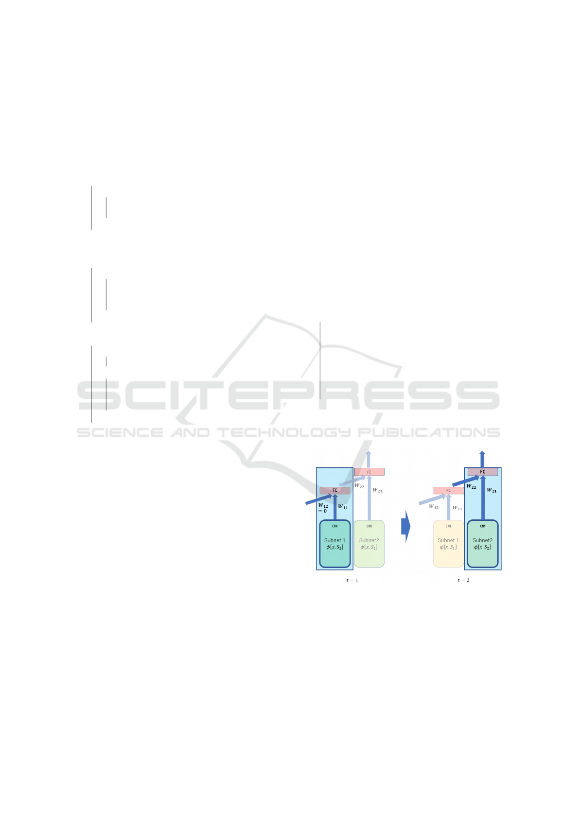
4.3 Adjusting the Aggregation Layer

After learning the subnetwork, the aggregation layer

is adjusted to ﬁt the ﬁnal output. The aggregation

layer consists of a fully-connected linear layer, and

is used to re-adjust the old sub-network output with-

out changing the old sub-network parameters. Let Y

be the i-th aggregation layer outputs, then

≡ ReLU



i−1



, (9)

where y

and Y

i−1

denote the i-th sub-network output

vector and the i −1-th ﬁnal output vectors, respec-

tively. W

and W

are the weight vectors connected

to the i-th sub-network output and the i −1-th ﬁnal

output vectors, respectively (see Fig 2). Then, the ﬁ-

nal classiﬁcation output is

c = argmax

i j

}, (10)

where Y

= [Y

,···Y

]

This layer is adjusted as follows

= W

−η(t)∇

aggregation

(11)

= W

−η(t)∇

aggregation

(12)

where η(t) is an adaptive learning rate controlled by

Adagrad (Luo et al., 2019), L

aggregation

denotes mean

square error loss given as

aggregation

≡

∑

t∈χ

∪χ

old

∥Y

−y

∥

(13)

Data: x

Result: Y

subnet

for i = 1 to N

subnet

S = load(S

) //load S

from the

secondary storage

= load(W

)

= load(W

)

←− φ(x,S) // calculate the i-th

subnetwork.

≡ ReLU



i−1



end

return Y

subnet

Algorithm 2: Pseudo code for inference.

Figure 2: Example of inference phase behavior.

5 POWER-CONSUMPTION

ANALYSIS

We assume the power-consumption P is proportional

to the computational complexity. So, we estimate P

from the complexity. Each sub-network uses only

some parameters with the top k scores, reducing P by:

ICPRAM 2024 - 13th International Conference on Pattern Recognition Applications and Methods

422

1. Less multiplication of weights and inputs.

2. Less setup for weights. The system only acti-

vates some weight connections, not sending pa-

rameters.

We consider the demands in table2.

Table 2: Notations for analysing power consumption.

item notation

Select the top k score connections. P

select

Calculation of the t-th sub-network

for a single input vector.

Csub

(t)

Calculation of the t-th aggregation-

layer for a single input vector.

Cagg

(t)

Learning of the t-th sub-network for

getting the top k scores.

Lsub

(t)

Learning of the t-th aggregation-

layer.

LAgg

(t)

5.1 Forward Calculation

The electricity of forward calculation for the t-

th sub-network and corresponding aggregation layer

f orward

(t) can be represented recursively as follows.

f orward

(t) = P

Cagg

(t) + P

Csub

(t) + P

f orward

(t −1)

(14)

where P

Cagg

(t) is the calculation cost for t-th ag-

gregation layer. P

Cagg

(t) depends on the number of

output connections of t = 1 ···T sub-networks. In

the t-th round, the aggregation layer’s input size is

t ×m, where m is the output size of each sub-network.

Therefore, if the number of classes is N

(output size

of the ﬁnal layer), the electricity for calculating the

aggregation layer is

Cagg

(t) =



m ·N

t = 1

2 ·m ·N

t ≥2

(15)

Therefore, we obtain

f orward

(t) = m ·N

(2t −1) +

∑

i=1

Csub

(t), (16)

where P

Csub

(t) depends on the number of the active

connections, Each sub-network is formed by select-

ing the top k connections. The selected connections

are set to active and the others are set to inactive. This

process wastes a lot of electrical power by sending

the information of the k connection indexes to the de-

vice. This process wastes P

select

= kν

send

where ν

send

denotes a positive coefﬁcient for sending data. From

this, the sub-network wastes

Csub

(t) = P

select

+ kν

(17)

= k(ν

send

+ ν

where ν

denotes a positive coefﬁcient, which de-

pends on the network structure. Therefore,

f orward

(t) = m ·N

(2t −1) +tk(ν

send

+ ν

), (18)

5.2 Learning

The electricity for the learning of the t-th sub-network

and the t-th aggregation layer P

learning

(t) is repre-

sented by

learning

(t) = P

Lsub

(t) + P

Lagg

(t). (19)

The power consumption for the learning sub-

network P

Lsub

(t) depends on the number of parame-

ters in the device N

device

and the number of samples

for the t-th round N

samples

(t).

Lsub

(t) = N

samples

(t)N

epoch

device

(20)

where ν

denotes a positive coefﬁcient for the learning

that is related to the network structure, N

epoch

is the

number of epochs. Note that the learning process also

includes the calculation process. We assume that ν

also includes the calculation cost, which is executed

during the learning.

The power consumption for the learning aggrega-

tion layer P

Lagg

(t) is

Lagg

(t) = N

samples

(t) ·N

epoch

(t ·m ·N

+ P

f orward

(t −1)),

(21)

Therefore,

learning

(t) = N

samples

(t)N

epoch

device

(22)

+ t ·m ·N

+ P

f orward

(t −1)



5.3 Power-Consumption vs # of

Sub-Networks

The power consumption for the forward calculation

5.1 and the learning 5.2 are O(t) for the t-th round.

In the t-th round, the total number of sub-networks

is t. This means that there is a trade-off between

the power-consumption and the ability of the sys-

tem, which increases by growing the number of sub-

networks. This also means that the system should

limit the number of sub-networks to a certain number

to reduce the power consumption.

6 EXPERIMENTS

Two experiments were conducted in this study. The

ﬁrst experiment involved checking the proposed net-

work Swap-NN for incremental learning tasks using

the MNIST dataset. The MNIST dataset was divided

into two or ﬁve sub-datasets.

Swap-Deep Neural Network: Incremental Inference and Learning for Embedded Systems

423

The second experiment involved checking the per-

formance of the Swap-NN for the large-scale learning

tasks. The CIFEAR-10 dataset was used to achieve

this. The CIFEAR-10 was divided into 2 subdatasets,

and Swap-NN repeated the learning 2 times.

6.1 Experiment for MNIST Dataset

We developed our program-code based on a sample.

https://github.com/allenai/hidden-networks/

simple_mnist_example.py

The size of each layer is the same as that of the origi-

nal program as listed in Table 3.

Table 3: Network size for MNIST: ’Conv’, ’fc’, ’C’, ’RF’

and ’ f [·] denote convolution layer, full-connection layer,

channel, receptive ﬁeld and activation function respectively.

’fc2:L’ and ’fc2:R’ denote the fc2 layer for the learning and

recognition, respectively.

Layer Input size C RF f [·]

Conv1 28 × 28 32 3 × 3 ReLU

Conv2 28 × 28 × 32 64 3 × 3 ReLU

MaxPool 28 × 28 64 2 × 2 –

fc1 1 × 9216 128 – ReLU

fc2:L 1 × 128 10 – Linear

fc2:R ReLU

It should be noted that non of the convolution or

fully-connecting layers have bias terms. The ReLU

was used as the activation function(Krizhevsky et al.,

2012). The initialization of each weight strength w

for the l-th layer was set using the Kaiming-normal

distribution(He et al., 2015) D

= N (0,

2/n

l−1

where n

l−1

denotes the number of inputs from the

previous layer. In contrast, the initial scores s

were

sampled uniformly from the set {−

√

5}.

6.1.1 Set Up of the Learning Samples

To evaluate the incremental learning ability of the pro-

posed method, its accuracy was evaluated for the test

samples after each incremental learning phase.

To this end, we used split MNIST, in which the

MNIST was divided into several groups. For exam-

ple, if MNIST was divided into two groups, the ﬁrst

group was the set of samples for labels {0,1,2,3,4},

and the second group was the set of samples for la-

bels {5,6,7,8,9}. During each incremental learning

phase, samples from a speciﬁc group were presented.

6.1.2 Evaluation

The learning task used in this paper corresponds

to ’incremental-class learning’ in the literature (Hsu

et al., 2018). We compared SwapNN’s performances

with those of the other methods on ’incremental-class

learning’ listed in (Hsu et al., 2018). After the last

incremental learning phase, the accuracy was eval-

uated using all test samples. If the learning ma-

chine causes the catastrophic forgetting due to the in-

cremental learning, the accuracy after the last incre-

mental learning will be low. If the learning method

yielded an accuracy of approximately 100× index of

the incremental learning phase/total number of incre-

mental learning, the learning method had achieved the

desired results.

6.1.3 Results

Preliminary results are shown in Table 4, This table

shows the accuracy of our proposed system, Swap-

NN, and other learning methods after learning the

MNIST dataset, which is divided into ﬁve sub-groups.

The table also shows the accuracy of other learning

methods: EWC (Kirkpatrick et al., 2017), SI (Zenke

et al., 2017) , Naive-rehearsal (Hsu et al., 2018) ,

MAS (Aljundi et al., 2018) and LwF (Li and Hoiem,

2016) , which are the same as the data reported in

(Hsu et al., 2018). Additionally, we list the Swap-NN

with two subnetworks, which learns MNIST divided

into two groups, at the bottom of the table.

The hyper parameter k of Swap-NN, which is the

number of the most important connections for yield-

ing the output, was set to k = κ ×N

device

. Note that

κ(< 1) denote the ratio and κ = 0.7. The replay-buffer

size B of Swap-NN was set to 12000. The Swap-NN

that learned ﬁve classes par each incremental learning

phase showed the highest accuracy (see the bottom of

Table 4).

We evaluated the memory consumption and com-

putational complexity of the models. The network

size of the competing models except Swap-NN was

almost the same, and the number of variable weight

parameters was 1708446. The total number of weight

connections in Swap-NN was 1199648. However,

Swap-NN used κ× 1199648 connections to com-

pute a single subnetwork output for the current input.

Therefore, in the case of the Swap-NN having two

subnetworks, it uses 2 ×κ×1199648 = 1679927 con-

nections to obtain the ﬁnal output. This number of

connections is not much different from the competing

models.

6.2 Experiment for CIFAR-10

Swap-NN was also tested for a more challenging

learning task by using CIFAR-10. CIFAR-10 dataset

was divided into two sub-datasets, thus each of the

two sub-datasets includes ﬁve classes dataset. The

network size is shown in Table 5, whose total number

ICPRAM 2024 - 13th International Conference on Pattern Recognition Applications and Methods

424

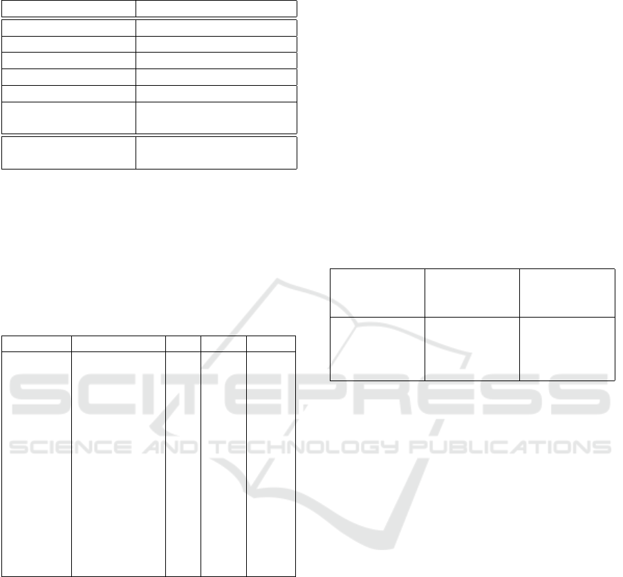
Table 4: Accuracy for MNIST dataset. The results reported

in (Hsu et al., 2018) are listed except those for Swap-NNs.

Method Incremental class learning

EWC 19.80 ± 0.05

SI 19.67 ± 0.09

MAS 19.52 ± 0.29

LwF 24.17 ± 0.33

Naive rehearsal 90.78 ± 0.85

Swap-NN (ﬁve sub-

networks)

90.92 ± 0.97

Swap-NN (two sub-

networks)

94.29 ± 0.32

of parameters are the same as that of the network used

in the previous experiment. Note that this network

size is relatively smaller than the normal network size

for the learning of CIFAR-10.

Table 5: Network size for CIFEAR-10: ’Conv’, ’fc’,’RF’,

’C’ and ’BN’ denote convolution layer, full-connection

layer , receptive ﬁeld, channel and batch-normalization

layer respectively. ’fc2:L’ and ’fc2:R’ denote the fc2 layer

for the learning and recognition, respectively.

Layer Input size C RF f [·]

Conv1 32 × 32 × 3 64 3 × 3 ReLU

Conv2 32 × 32 × 64 64 3 × 3 ReLU

BN1 32 × 32 × 64 64 – –

MaxPool1 32 × 32 64 2 × 2 –

Conv3 32 × 32 × 64 128 3 × 3 ReLU

Conv4 32 × 32 × 128 128 3 × 3 ReLU

BN2 32 × 32 × 128 128 – –

MaxPool2 32 × 32 128 2 × 2 ReLU

Conv5 32 × 32 × 128 256 3 × 3 ReLU

Conv6 32 × 32 × 256 256 3 × 3 ReLU

BN3 32 × 32 × 256 256 – –

MaxPool3 32 × 32 256 2 × 2 ReLU

fc1 1 × 4096 256 – ReLU

fc2:L 1 × 256 10 – Linear

fc2:R ReLU

We compare the Swap-NN performance with that

of the same sized neural network, which has learned

all training samples of the CIFAR-10. The perfor-

mances of the both networks after ﬁnishing the learn-

ing were evaluated by using the validation set in the

CIFAR-10. The test was repeated 10 times by chang-

ing the initial weight connections randomly. The re-

sults were averaged over the 10 trials and 95 percent

conﬁdence intervals were also estimated.

6.2.1 Results

The buffer size B was set to 20000.

We compared the accuracy rate of SwapNN,

which learned ﬁve classes at a time, with that of a

network that learned all classes simultaneously, un-

der the same conditions with those of SwapNN (the

same network size and 5 epochs). Table 6 shows the

accuracy after the initial and incremental learning.

This result suggests that the accuracy of our pro-

posed SwapNN is about 5.3 points less than the net-

work, which learns all classes at a time. However,

after the initial learning, the accuracy for the 1st ﬁve

classes was 79.8 %. Each subnetwork has no opportu-

nity to learn the class boundaries between the future

presented classes. Therefore, each subnetwork out-

put will conﬂict to the future unknown classes. To

overcome this problem, the last aggregation layer has

to adjust to this kind of mismatch. However, there are

possibility that the last aggregation layer could not ad-

just this conﬂict completely in the case of CIFAR10.

Table 6: 95% conﬁdence interval of SwappNN accuracy af-

ter each incremental learning on CIFAR-10 (The ’Competi-

tor’ is the network that learned all classes at once.).

After initial

learning

After the

incremental

learning

Competitor

39.42 ± 0.20

% (79.8%

for learned 5

classes)

65.09 ± 1.17

70.95 ± 0.53

7 DISCUSSION

7.1 Computational Complexity vs

Accuracy

Obviously, the computational complexity is low if k is

small. Instead of the light weight computation of the

sub-network, the proposed method has to repeat the

setup of the sub-network and calculation of the sub-

network. To reduce the computation time, k should be

small enough to realize a quick computation. How-

ever, too small k will yield the degradation of the per-

formance.

7.2 Suitable Learning Strategy for Each

Sub-Network

In the classiﬁcation tasks, each sub-network should

learn the class-boundaries. Without the information

for the boundaries, the learning machine will fail to

acquire a high performances. So, the number of

classes, of which the learning samples presented dur-

ing an incremental learning phase, should be large.

The connection set found in each learning phase

are stored in the second storage device and ﬁxed so

Swap-Deep Neural Network: Incremental Inference and Learning for Embedded Systems

425

far. However, the connection set should be updated

when environment is changed. The distillation strat-

egy employed in Foster (Wang et al., 2022) is also

useful for reducing and re-adjusting the subnetworks.

The distillation operation will give a clear opportunity

to make each subnetwork and corresponding aggrega-

tion layer learn class boundaries.

8 CONCLUSION

In this paper, a hidden neural network based incre-

mental learning method: Swap deep neural network

is proposed. This model has been followed two ad-

vantages:

1. The hidden neural network can reuse its neurons

in several different tasks by reconﬁguration of the

neural network circuit. So, this architecture is

suitable for a small embedded systems, where the

storage capacity is limited.

2. The sub-network is not modiﬁed after the cre-

ation. This means that the system does not cause

the catastrophic forgetting.

The simulation results suggest that Swap-NN re-

alizes an effective execution of large-scale neural net-

works with a small amount of resources.

REFERENCES

Aljundi, R., Babiloni, F., Elhoseiny, M., Rohrbach, M.,

and Tuytelaars, T. (2018). Memory aware synapses:

Learning what (not) to forget. In Proceedings of

the European Conference on Computer Vision (ECCV

2018).

French, R. M. (1997). Pseudo-recurrent connectionist

networks: An approach to the “sensitivity stability”

dilemma. Connection Science, 9(4):353–379.

French, R. M. (1999). Catastrophic forgetting in connec-

tionist networks. TRENDS in Cognitive Sciences,

3(4):128–135.

Freund, Y. and Schapire, R. E. (1997). A decision-theoretic

generalization of on-line learning and an application

to boosting. Journal of Computer and System Sci-

ences, 55(1):119–139.

Fukushima, K. (1975). Cognitron: A self-organizing mul-

tilayered neural network. Biological Cybernetics,

20(3):121–136.

Hayes, T. L., Kaﬂe, K., Shrestha, R., Acharya, M., and

Kanan, C. (2019). Remind your neural network to

prevent catastrophic forgetting. CoRR.

He, K., Zhang, X., Ren, S., and Sun, J. (2015). Delving

deep into rectiﬁers: Surpassing human-level perfor-

mance on imagenet classiﬁcation. In 2015 IEEE In-

ternational Conference on Computer Vision (ICCV),

pages 1026–1034.

Hinton, G., Vinyals, O., and Dean, J. (2015). Distilling the

knowledge in a neural network. arXiv.org.

Hirose, K., Yu, J., Ando, K., Okoshi, Y., Garc

ıa-Arias,

A. L., Suzuki, J., Chu, T. V., Kawamura, K., and Mo-

tomura, M. (2022). Hiddenite: 4k-pe hidden network

inference 4d-tensor engine exploiting on-chip model

construction achieving 34.8-to-16.0tops/w for cifar-

100 and imagenet. In 2022 IEEE International Solid-

State Circuits Conference (ISSCC), volume 65, pages

1–3.

Hsu, Y.-C., Liu, Y.-C., Ramasamy, A., and Kira, Z. (2018).

Re-evaluating continual learning scenarios: A cate-

gorization and case for strong baselines. In Ben-

gio, S., Wallach, H., Larochelle, H., Grauman, K.,

Cesa-Bianchi, N., and Garnett, R., editors, Advances

in Neural Information Processing Systems 31. Curran

Associates, Inc.

Ishikawa, M. (1996). Structural learning with forgetting.

Neural Networks, 9(3):509–521.

Kirkpatrick, J., Pascanu, R., Rabinowitz, N., Veness, J.,

Desjardins, G., Rusu, A. A., Milan, K., Quan, J., and

Ramalho, T. (2017). Overcoming catastrophic forget-

ting in neural networks. Proceeding of the National

Acacemy of United States of America, 114(13):3521–

3526.

Krizhevsky, A., Sutskever, I., and Hinton, G. E. (2012).

Imagenet classiﬁcation with deep convolutional neu-

ral networks. In Pereira, F., Burges, C. J. C., Bottou,

L., and Weinberger, K. Q., editors, Advances in Neu-

ral Information Processing Systems 25, pages 1097–

1105. Curran Associates, Inc.

Li, Z. and Hoiem, D. (2016). Learning without forgetting.

In European Conference on Computer Vision 2016,

pages 614–629. SCITEPRESS ? Science and Technol-

ogy Publications, Lda.

Luo, L., Xiong, Y., Liu, Y., and Sun, X. (2019). Adap-

tive gradient methods with dynamic bound of learning

rate. In International Conference on Learning Repre-

sentations ICLR2019.

Mallya, A. and Lazebnik, S. (2018). Packnet: Adding mul-

tiple tasks to a single network by iterative pruning.

In CVPR, Conference on computer vision and pattern

recognition 2018, pages 7765–7773.

Ramanujan, V., Wortsman, M., Kembhavi, A., Farhadi, A.,

and Rastegari, M. (2020). What’s hidden in a ran-

domly weighted neural network? arXiv.org.

Rusu, A. A., Rabinowitz, N. C., Desjardins, G., Soyer,

H., Kirkpatrick, J., Kavukcuoglu, K., Pascanu, R.,

and Hadsell, R. (2016). Progressive neural networks.

CoRR.

Sadel, J., Kawulok, M., Przeliorz, M., Nalepa, J., and

Kostrzewa, D. (2023). Genetic structural nas: A neu-

ral network architecture search with ﬂexible slot con-

nections. In GECCO’23 Companion: Proceedings of

the Companion Conference on Genetic and Evolution-

ary Computation, pages 79–80. Association for Com-

puting Machinery.

Wang, F.-Y., Zhou, D.-W., Ye, H.-J., and Zhan, D.-C.

(2022). Foster: Feature boosting and compression

for class-incremental learning. In ECCV 2022: 17th

ICPRAM 2024 - 13th International Conference on Pattern Recognition Applications and Methods

426

European Conference, Proceedings, Part XXV, pages

398–414.

Yamauchi, K., Yamaguchi, N., and Ishii, N. (1999). In-

cremental learning methods with retrieving interfered

patterns. IEEE TRANSACTIONS ON NEURAL NET-

WORKS, 10(6):1351–1365.

Zenke, F., Poole, B., and Ganguli, S. (2017). Continual

learning through synaptic intelligence. In Proceed-

ings of the 34th International Conference on Machine

Learning, Sydney, Australia, PMLR 70, 2017.

Zheng, N. and Mazumder, P. (2020). Learning in Energy-

Efﬁcient Neuromorphic Computing: Algorithm and

Architecture Co-Design. John Wiley & Sons Inc.

Swap-Deep Neural Network: Incremental Inference and Learning for Embedded Systems

427