Enhancing Portfolio Performance: A Random Forest Approach to

Volatility Prediction and Optimization

Vedant Rathi

1 a

, Meghana Kshirsagar

2 b

and Conor Ryan

2 c

Adlai E. Stevenson High School, Lincolnshire, U.S.A.

Biocomputing Developmental Systems Research Group, Department of CSIS, University of Limerick, Limerick, Ireland

Keywords:

Volatility Prediction, Portfolio Optimization, Machine Learning, Random Forest, Investing Techniques.

Abstract:

Machine learning has diverse applications in various domains, including disease diagnosis in healthcare, user

behavior analysis, and algorithmic trading. However, machine learning’s use in portfolio volatility predictions

and optimization has only been recently explored and requires further investigation to prove valuable in real-

world settings. We thus propose an effective method that accomplishes both these tasks and is targeted at

people who are new to the realm of ﬁnance. This paper explores (a) a novel approach of using supervised

machine learning with the Random Forest algorithm to predict portfolio volatility value and categorization

and (b) a ﬂexible method taking into account users’ restrictions on stock allocations to build an optimized

and customized portfolio. Our framework also allows a diversiﬁed number of assets to be included in the

portfolio. We train our model using historical asset prices collected over 8 years for six mutual funds and

one cryptocurrency. We validate our results by comparing the volatility predictions against recent asset prices

obtained from Yahoo Finance. The research underlines the importance of harnessing the power of machine

learning to improve portfolio performance.

1 INTRODUCTION

Portfolio management refers to the science of select-

ing investment types that meet the ﬁnancial objec-

tives of a client. Typically, these objectives involve

a combination of maximizing performance and min-

imizing risk. Portfolio management is critical as in-

stitutions need to meet ﬁnancial obligations daily, to

satisfy their own goals and the goals of individuals

who are in some way connected to such institutions.

Despite a wide variety of portfolio tools being

freely available for use, the vast majority of investors

fail to earn portfolio returns that exceed the market

rate. Many studies attribute this phenomenon to a

lack of diversiﬁcation, herd behavior, and the efﬁcient

market hypothesis, leading to sub-optimal portfolio

performance.

Diversiﬁcation of investment types is one of the

most widely known investment strategies. It refers

to spreading one’s investments across different asset

classes to protect one’s portfolio against adverse mar-

https://orcid.org/0009-0009-3300-1820

https://orcid.org/0000-0002-8182-2465

https://orcid.org/0000-0002-7002-5815

ket movements. However, many falsely believe that

having investments in many asset classes will aug-

ment volatility levels (Reinholtz et al., 2021).

Herd behavior, where individuals mimic the ac-

tions of a larger group rather than making independent

decisions, can lead to market bubbles as investors col-

lectively rush to buy assets, driving up prices without

individual asset analysis (Choijil et al., 2022).

Lastly, the efﬁcient market hypothesis states that

all available market information is reﬂected in as-

set prices, thus suggesting that, in theory, investors

shouldn’t be able to achieve above-average returns

consistently (Mancuso, 2022).

This paper proposes a model to help investors

overcome these challenges and enhance portfolio per-

formance. Our main contributions are two-fold. First,

we use the Random Forest algorithm to predict the

volatility of a random portfolio (with a variety of in-

vestment types), helping to quantify the risk for a cer-

tain portfolio and imply suggestions about diversiﬁ-

cation for an investor. Second, we perform portfolio

optimization while allowing users to include their in-

vestment allocation restrictions to augment the overall

ﬂexibility.

1278

Rathi, V., Kshirsagar, M. and Ryan, C.

Enhancing Portfolio Performance: A Random Forest Approach to Volatility Prediction and Optimization.

DOI: 10.5220/0012464600003636

Paper published under CC license (CC BY-NC-ND 4.0)

In Proceedings of the 16th International Conference on Agents and Artiﬁcial Intelligence (ICAART 2024) - Volume 3, pages 1278-1285

ISBN: 978-989-758-680-4; ISSN: 2184-433X

2 RELATED WORKS

Machine learning is a widely used technique for port-

folio optimization (Bartram et al., 2021) and volatil-

ity prediction or forecasting. Our work derives from

the portfolio-related ML contributions that other re-

searchers have conducted.

Kobets et al. (Kobets and Savchenko, 2022) ex-

plores the use of long short-term memory neural net-

works and linear regression models to create an opti-

mal portfolio based on price predictions, ﬁnding that

taking into account one-month asset prices improved

their performance results. They used the Markowitz

portfolio model (modern portfolio theory) to optimize

the portfolio, which was trained using historical data,

similar to what we did.

Ma et al. (Ma et al., 2020) similarly analyze the

effectiveness of three different types of deep neu-

ral networks in portfolio optimization. They chose

semi-absolute deviation as the risk indicator, which

involves calculating the absolute differences between

data points and the central measure, whereas varia-

tion involves the squares of these differences. Our

study predicted volatility, which is the square root of

variation.

Another LSTM-involved portfolio recommenda-

tion system was by Leung et al. (Leung et al., 2023),

who used a web application to take into account user

preferences in their optimization algorithm. We also

included a feature with user involvement in our opti-

mization method.

A recent study involving reinforcement learning

(Gao et al., 2021) used Deep Q-Network for portfo-

lio management to take into account transaction fees.

They measured the cumulative rate of returns for the

portfolio. Their model was ﬂexible to accommodate

any number of assets, similar to ours.

Furthermore, a literature review (Ertenlice and

Kalayci, 2018) ﬁnds that variance tends to be the most

commonly used risk indicator and Markowitz’s mean-

variance portfolio theory to be the most commonly

used formulation for portfolio optimization. In line

with these prevailing practices, we also used these two

methods in our study, thus fortifying the robustness of

this research.

While most research discusses new portfolio op-

timization techniques, machine learning is also used

for volatility forecasting. Christensen et al. (Chris-

tensen et al., 2021) ﬁnd that machine learning tech-

niques outperform the HAR (heterogeneous autore-

gressive) model. However, with this in mind, most

volatility predictive models involve a temporal aspect,

such as intraday volatility forecasting. Zhang et al.

(Zhang et al., 2022) employs neural networks to fore-

cast volatility over very short-term periods such as 10

or 30 minutes. Our research instead predicts annual-

ized volatility given random asset allocations.

The majority of the literature covered only uses

ML techniques to optimize their portfolio; however,

our research uses ML to predict volatility and uses

modern portfolio theory with ML to optimize a port-

folio. Furthermore, to the best of our knowledge, the

dataset we tested our model on was the historical as-

set prices of mutual funds (and one cryptocurrency),

which we believe to be a novelty.

Finally, predicting market volatility using the Ran-

dom Forest model has been vastly unexplored. De-

spite this fact, Kumar et al. (Kumar et al., 2018)

showed that Random Forest tends to perform the best

at predicting stock market activity for large datasets

out of ﬁve supervised machine learning models stud-

ied, justifying our use of this model. Cervell

o-Royo et

al. (Cervell

o-Royo and Guijarro, 2020) similarly con-

cluded Random Forest’s superior capabilities in pre-

dicting stock market movement compared to the other

ML methods in the study.

3 ASSUMPTIONS

Before we introduce and explain our model, we make

the following assumptions:

• Measuring the volatility of a portfolio is a sufﬁ-

cient and suitable metric to gauge the risk level of

such a portfolio.

• The bounds for the generated random allocations

of the assets (e.g. metal, cryptocurrency, etc.) in

our data set represent common investment prac-

tices and recommendations (Liu and Tsyvinski,

2021).

• Sharpe Ratio assumes a constant risk-free rate

(Sharpe, 1998), which may not reﬂect real market

conditions.

• The Random Forest model is a suitable choice

for this study based on its interpretability, robust

performance, and well-researched ability to han-

dle various data types. While much other re-

search uses neural networks, we ﬁnd Random For-

est most appropriate for our scenario.

• The features used in the RF model are representa-

tive of the factors affecting portfolio volatility.

Enhancing Portfolio Performance: A Random Forest Approach to Volatility Prediction and Optimization

1279

Table 1: Summary of Volatility Prediction Approaches.

Author(s) Model Used Dataset

(Vidal and

Kristjan-

poller, 2020)

Convolutional Neural Networks with Long Short-Term Memory

(CNN-LSTM)

Gold Market

(Idrees et al.,

2019)

Autoregressive Integrated Moving Average (ARIMA) Indian Stock

Market

(Hu et al.,

2020)

Generalized Autoregressive Conditional Heteroskedasticity

(GARCH), Long Short-Term Memory with Artiﬁcial Neural

Networks (LSTM-ANN)

Copper Market

(Kim and

Won, 2018)

Long Short-Term Memory, Generalized Autoregressive Condi-

tional Heteroskedasticity (GARCH)

KOSPI (200 Ko-

rean stocks)

(Walther

et al., 2019)

Generalized Autoregressive Conditional Heteroskedasticity

variant of Mixed Data Sampling (GARCH-MIDAS)

CRIX (Cryp-

tocurrency

index) and ﬁve

high-revenue

cryptocurrencies

(Hwang and

Hong, 2021)

Multivariate Heterogeneous Autoregressive-Realized Volatil-

ity model with Generalized Autoregressive Conditional Het-

eroskedasticity (HAR-RV-GARCH)

S&P 500 Index,

KOSPI, Russell

2000, and EURO

STOXX 50

(Wen et al.,

2016)

16 HAR (Heterogeneous Autoregressive)-type models WTI (West Texas

Intermediate)

Crude Oil Fu-

tures

4 PROBLEM METHODOLOGY

4.1 Overview

We will now provide a brief overview of our research

methodology. We began by identifying the problem,

noting that much of the research on volatility pre-

diction and portfolio optimization is relatively recent;

hence, new methods for performing these tasks should

be explored. Next, we collect the data with a Python

library, allowing access to historical prices for assets.

After collection, we process the data to ﬁlter it such

that only the information needed is kept, and we pre-

pare it to be read by our model. Once the data is

fully cleaned, we feed it into our model, the major-

ity of which is used for training and the rest for test-

ing. Next, we use our model for volatility prediction

and portfolio optimization. Finally, we evaluate our

model performance and make any tweaks as neces-

sary.

Next, we look at other research approaches that

accomplished a similar task as our research for

volatility prediction. The majority of the studies in

Table 1 show the following two commonalities:

• The use of neural networks or time-series related

models. CNN and ANN are neural networks,

while ARIMA and GARCH are employed for

time-series data.

• The dataset tends to be an entire market in either

one geographic area or encompassing one asset

type.

Our research is unique in that we use Random For-

est for volatility prediction (which is much less ex-

plored). Furthermore, our dataset spans a variety of

asset types and isn’t restricted to one geographic area.

Table 2 compares our approach for portfolio op-

timization to other methods. We note that while us-

ing mean-variance optimization was a commonality

among most approaches, few used the Random For-

est model as well and included a cryptocurrency in

the data set used for training.

The Random Forest model is an ensemble learn-

ing method, where multiple instances of a base learn-

ing algorithm, speciﬁcally decision trees, are em-

ployed to enhance the model’s predictive capabili-

ties. This comes with numerous advantages over

other models, including a smaller likelihood of over-

ﬁtting (when an ML model generates accurate results

for the training data set but not for testing) and im-

proved accuracy. These two factors and other advan-

tages of RF also improve its interpretability.

We thus argue that our model has high inter-

ICAART 2024 - 16th International Conference on Agents and Artiﬁcial Intelligence

1280

Table 2: Comparison of Machine Learning-based Portfolio

Optimization Methods.

Author(s) Model Crypto

cur-

rency

Mean-

Variance

Opti-

mization

(Ma et al.,

2021)

RF, SVR,

LSTM,

CNN &

MLP

× ✓

(Chen et al.,

2021)

XGBoost

& IFA

× ✓

(Aboussalah

and Lee,

2020)

SDDRRL ? ×

Our model RF ✓ ✓

pretability, referring to the extent to which humans

can predict a model’s outcome and understand the

method by which the outcome was produced (Eras-

mus et al., 2021). For example, given a higher allo-

cation of cryptocurrency, our model will predictably

output a higher volatility value compared to a smaller

allocation. In contrast to black-box models, our Ran-

dom Forest model predicts portfolio risk given certain

asset allocations, making its decision-making process

very understandable. The features and target variables

are carefully selected. We can also dissect the deci-

sion trees that the ML model used to get a breakdown

of how the model reached a certain risk assessment.

Each node in the decision tree represents a decision

point, and one’s ability to easily trace this tree-based

structure improves our model’s interpretability.

While a single decision tree is inherently more

interpretable than multiple decision trees, this may

come at the cost of capturing more nuanced patterns

and trends in the data provided. Therefore, we choose

to balance transparency and complexity to provide a

more robust prediction mechanism while still being

highly interpretable.

4.2 Data Set

For our Random Forest model, we used the following

seven tickers: VTSAX, VTIAX, VBTLX, VDE, VGSLX,

OPGSX, and BTC-USD. Note that the ﬁrst six are

mutual funds, and the last ticker is a cryptocurrency.

These seven tickers cover a wide range of investment

types, i.e., real estate, stocks, bonds, etc. We col-

lected historical ticker prices over an 8-year range

(from 2015 to 2023) using the yﬁnance Python API

(which uses Yahoo Finance market data). Using the

asset prices, we found the daily returns (percentage

Figure 1: Distribution of Data Set Asset Daily Returns.

change in price for consecutive days) as follows:

Daily Returns =

−P

k−1

(1)

where P

denotes the price of an asset at day k. From

Figure 1, we can visualize the daily returns distribu-

tions (encompassing all eight years of data) for each

of the seven tickers.

4.3 Data Architecture

To transform the data into a form in which our model

could predict volatility, we created 5000 random in-

stances of possible ticker allocations. Each instance

has the following criteria:

+ w

= 1 (2)

≥ 0, i ∈{1, 2, 3, 4, 5, 6, 7} (3)

≤ 0.20, w

≤ 0.10 (4)

where w

denotes the ticker weight (allocation

amount) for ticker i. w

, w

, and w

refer to the weights of tickers VTSAX, VTIAX, VBTLX,

VDE, VGSLX, OPGSX, and BTC-USD, respectively.

Our model is still compatible without the restrictions

on w

, w

, and w

, but we choose to include them

to better represent common real-life investment prac-

tices.

For each one of these 5000 random allocations,

we found the dot product of the daily returns with

the allocations, calculated the standard deviation (the

statistical measure of market volatility) of these dot

products, and annualized this standard deviation:

= r

·w

+ r

·w

+ ···+ r

·w

= r

·w

+ r

·w

+ ···+ r

·w

= r

·w

+ r

·w

+ ···+ r

·w

(5)

Here d

denotes the dot product of the returns r

and

weight w

for a certain day n and asset i. Next, to

Enhancing Portfolio Performance: A Random Forest Approach to Volatility Prediction and Optimization

1281

calculate the annualized volatility, we can do the fol-

lowing:

µ =

∑

i=1

(6)

∑

i=1

−µ)

(7)

= σ

√

252 (8)

We multiply the daily volatility, σ

, by the square

root of 252 to obtain the annual volatility, σ

, because

there are approximately 252 trading days in a year.

We repeat these calculations for 5000 random alloca-

tions to obtain the annualized volatility for 5000 in-

stances.

Next, we sort the annualized volatility values from

increasing to decreasing order. Using the sorted

values, we categorize the volatility values based on

quartiles, in which the largest 25% are classiﬁed as

“High”, the second-largest as “Moderate,” the second-

smallest as “Medium”, and the smallest 25% as

“Low”.

We obtained Table 3 for the lower and upper

bounds of our risk categorization. Note that while our

Table 3: Volatility Bounds by Risk Category.

Risk Category Lower Bound Upper Bound

Low 0% 6.389%

Medium 6.390% 9.323%

Moderate 9.324% 12.656%

High 12.657% ∞

data produced a minimum volatility value of 3.856%

and a maximum value of 24.540%, the actual volatil-

ity values could theoretically range from 0% to an ex-

tremely high volatility value, so we thus adjust our

table accordingly.

4.4 Random Forest Model

We employed a Random Forest classiﬁer and re-

gressor to predict the volatility value category and

amount, respectively. Both algorithms use an 80-20

split in which 80% of the data is used for training

the model and 20% for testing, as empirical studies

show that allocating 20% to 30% of data for testing

results in optimal model performance (Dunford et al.,

2014). In other words, 4000 random allocation in-

stances were used for the training data set, and the

remaining 1000 for the testing set. For the classiﬁer,

the input features were the instances of random asset

allocations, and the target variable was the risk rat-

ing. The regressor had the same input features, but its

target variable was the annualized volatility value.

Figure 2: Random Forest Regressor Scatter Plot.

We also performed hyperparameter tuning using

an exhaustive grid search but found the changes in

model performance to be negligible. Our current

model has 100 estimators, no max depth, and 1 max

feature.

Figure 2 identiﬁes the regressor’s performance on

the testing data set. Our model consistently outputs a

predicted volatility which is very close in value to the

ideal prediction (actual volatility).

4.5 Additional Features

To improve the utility of our model’s predictive abili-

ties and make it more user-friendly, we created a fea-

ture allowing users to enter any number of portfolios

with their random allocations for the given assets. We

then rank the portfolios from highest volatility to low-

est volatility.

4.6 Portfolio Optimization

To optimize the portfolio, we use the Efﬁcient Fron-

tier model (Elton and Gruber, 1997), which is the set

of portfolios that either (a) maximize the returns of a

portfolio given a certain level of risk or (b) minimize

the risk of a portfolio given a certain level of returns.

To ﬁnd these sets of portfolios, we aim to maximize

the Sharpe Ratio given the set of constraints. The

Sharpe Ratio can be calculated as follows:

= (w

·r

) + (w

·r

) + ···+ (w

·r

)

(9)

∑

·w

·σ(R

(t)) ·σ(R

(t)) ·cov(R

(t), R

(t))

(10)

S =

E[R

−R

]

(11)

Here, R

represents the portfolio expected returns,

is the weight of asset i, r

is the expected returns for

asset i, σ

is the portfolio volatility, R

(t) is the time

series of returns for asset i, cov is the covariance of

ICAART 2024 - 16th International Conference on Agents and Artiﬁcial Intelligence

1282

two assets, R

is the risk-free rate, and S is the Sharpe

ratio (Pav, 2021).

The covariance of two assets can be calculated as

follows:

cov(R

(t), R

(t)) =

N −1

∑

k=1

) −

)(R

) −

)

(12)

where

represents the mean of R

(t).

The expected returns for asset i, which we call r

represents the compound annual growth rate (CAGR).

CAGR is calculated as follows:

= (P

−P

)

−1 (13)

and P

represent the initial and ﬁnal prices for asset

i and t is the number of years.

We let the user enter either a target maximum

volatility value or target minimum return value and

then provide them with the optimum portfolio using

this method. The user can also add their allocation

restrictions; for example, a user can include a con-

dition such that some ticker i has an allocation of at

least 20%, and the algorithm will consider this when

reoptimizing.

5 RESULTS

We ﬁrst present some performance metrics to mea-

sure the accuracy of our volatility-predicting Random

Forest model.

Table 4: Random Forest Performance Metrics.

RF Model Metric Type Value

Classiﬁer Accuracy Score 0.946

Regressor R-squared value 0.998

Regressor Mean Squared Error 3.80 ×10

−6

Based on Table 4, our model shows promising

strength as both the classiﬁer and regressor were over-

all accurate and precise.

Upon comparison of our RF model to a simple

ANN, we ﬁnd that the ANN performs slightly better

for volatility level classiﬁcation.

We also found the feature importances for the

regressor. The three most inﬂuential tickers were

VBTLX with 79.22% importance, VDE with 18.58%,

and BTC-USD with 1.36%. The other four tickers had

a combined importance of less than 1%.

Next, we compare our model to real-life data. We

access the most recent half-year’s worth of historical

asset prices to do so. We then repeat the following

steps for 1000 iterations:

1. Generate one sample of random weights

Figure 3: Random Forest Model Performance Versus

Current Data.

2. Calculate the actual annualized volatility from this

sample

3. Use the model to ﬁnd the predicted volatility

4. Find the absolute value of the differences between

the actual and predicted volatility values

We then found the average of these 1000 data points

to be 3.570%. Due to a lack of research using in-

dex funds as the primary allocation source of data,

we couldn’t conduct a fair comparison of the perfor-

mance of other models to ours. However, considering

this predicts annualized volatility, which would not

be used for high-frequency trading, we consider our

model a solid predictor.

Table 5 shows our model’s performance for three

randomly generated instances of portfolio allocations

for the weights of seven tickers speciﬁed in Subsec-

tion 4.3. All the values shown are in percentages.

Thus we see our model’s overall consistent perfor-

mance.

Figure 3 shows how our model is stronger at pre-

dicting portfolios of lower “actual” volatility than a

higher “actual” volatility, likely because portfolios

with higher volatility tend to be more unpredictable.

Next, looking at Figure 4, we see that the curved

line represents the optimal portfolios given a certain

level of maximum risk or minimum return. Here, we

deﬁne “efﬁcient risk” as the portfolio giving the min-

imum amount of risk for a certain level of expected

returns and “efﬁcient return” as the portfolio with the

maximum returns for a certain level of risk.

Note that we choose to show an example where

the user adds a certain asset weight restriction given

that their target risk level was 8% (orange circle);

hence, the Sharpe ratio for this portfolio, as calcu-

lated in Equation 9, was lower than without any re-

strictions (blue circle). The green triangle represents

another sample case where the user entered a target

Enhancing Portfolio Performance: A Random Forest Approach to Volatility Prediction and Optimization

1283

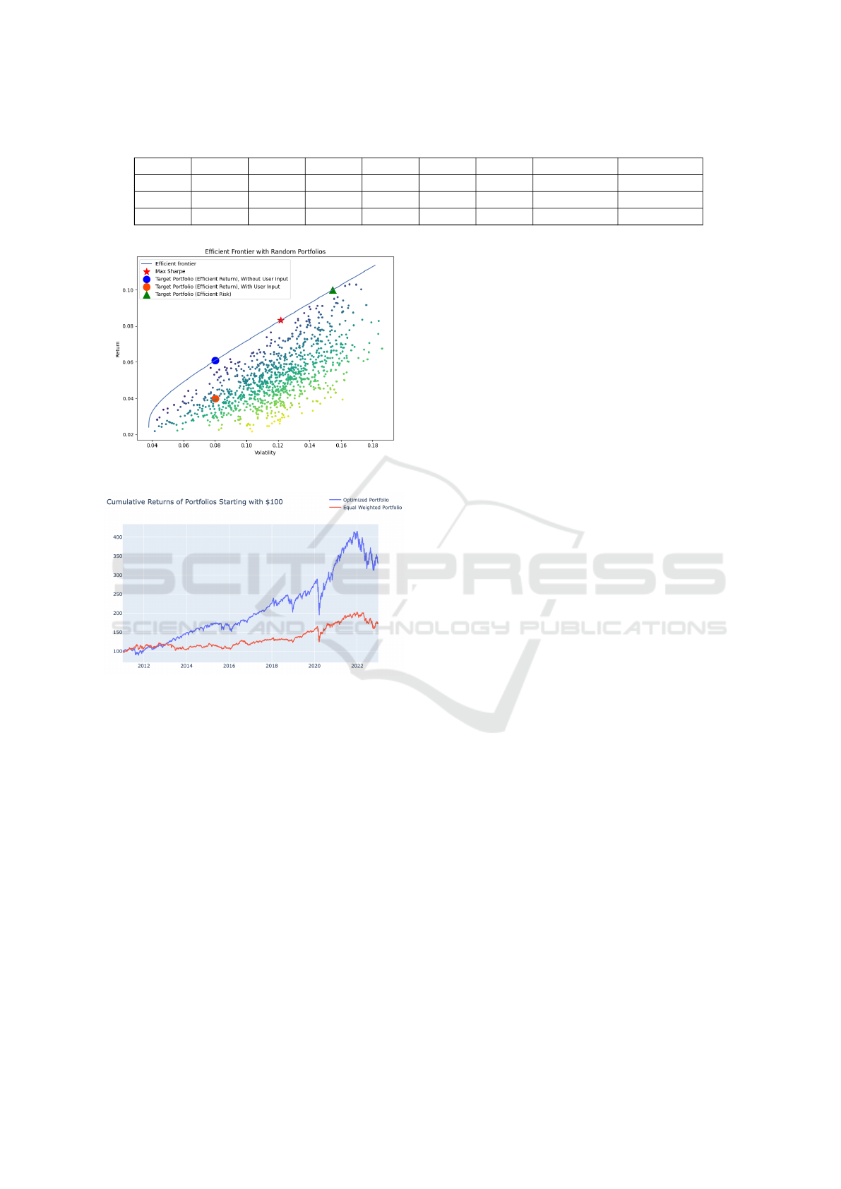
Table 5: Actual vs. Predicted Volatility for Three Random Portfolio Allocations (in Percentages).

Actual Predicted

2.56 17.67 51.04 12.63 4.78 9.16 2.16 8.07 10.35

6.54 24.15 32.26 8.77 10.84 17.24 0.20 10.02 12.82

0.55 1.84 79.93 7.57 3.47 0.69 5.95 6.82 6.98

Figure 4: Efﬁcient Frontier Portfolios Visualization.

Figure 5: Optimize Portfolio vs. Equal-Weighted Portfolio

Cumulative Returns.

return value of 10%.

From Figure 5, we see that our portfolio optimizer

performs nearly triply as strong as a generic, equal-

weighted portfolio in terms of cumulative return. The

optimized portfolio (blue line) represents the portfolio

with the seven tickers whose allocations maximize the

Sharpe Ratio. For the equal-weighted portfolio, each

ticker had an allocation of approximately 14.286%

(100/7), as we trained our model with seven tickers.

6 CONCLUSIONS AND FUTURE

WORK

In this paper, we present (a) a new method of predict-

ing volatility for a portfolio and create (b) a portfolio

optimizer that allows user input on the portfolio asset

allocations. Our data set consists of 7 tickers – 6 mu-

tual funds and one cryptocurrency. We use Yahoo Fi-

nance historical prices for data and ﬁnd that the mean

difference between our Random Forest volatility pre-

dictor and the actual volatility value is 3.570%. Fur-

thermore, our portfolio optimizer performs strongly

against a generic portfolio. We use modern portfolio

theory to do so, calculating the Sharpe Ratio while

considering user input.

First, the Efﬁcient Frontier assumes that invest-

ments generate returns that follow a primarily normal

distribution. However, this isn’t always true of the

market as the distribution often shows fat tails (Eom

et al., 2019), in which the likelihood of extreme events

occurring is higher than expected and predicted in

a normal distribution. Hence, this could impact our

model’s allocations after performing the portfolio op-

timization.

Second, our volatility-predicting model only uses

closing prices of assets from day to day, as this was

what was available through the Yahoo Finance API.

However, volatility can also be inﬂuenced by intra-

day price ﬂuctuations. Hence, our results may not

fully encompass the price changes relevant to differ-

ent time frames. This also limits the scope to which

our results can be generalized.

For future work, ﬁrst, we plan to incorporate as-

pects of neural networks (Sharkawy, 2020) with Ran-

dom Forest to strengthen the model. Using LSTM

will allow us to do a time-series analysis to capture

potential temporal factors involved in stock prices,

which we couldn’t accomplish with just Random For-

est. Neural networks also prove valuable with time

series forecasting.

Second, we also plan to build upon more mod-

ern portfolio optimization techniques including hier-

archical risk parity, the Black-Litterman model, and

Monte Carlo simulations. Mean-variance optimiza-

tion often leads to portfolios overly concentrated in

certain assets and may not adequately account for tail

risk. However, by implementing more modern mod-

els, we hope to consider a broader range of factors

that could affect stock market activity, including prob-

abilistic scenarios.

ICAART 2024 - 16th International Conference on Agents and Artiﬁcial Intelligence

1284

REFERENCES

Aboussalah, A. M. and Lee, C.-G. (2020). Continuous con-

trol with stacked deep dynamic recurrent reinforce-

ment learning for portfolio optimization. Expert Sys-

tems with Applications, 140:112891.

Bartram, S. M., Branke, J., De Rossi, G., and Motahari, M.

(2021). Machine learning for active portfolio manage-

ment. The Journal of Financial Data Science, 3(3):9–

30.

Cervell

o-Royo, R. and Guijarro, F. (2020). Forecasting

stock market trend: A comparison of machine learn-

ing algorithms. Finance, Markets and Valuation,

6(1):37–49.

Chen, W., Zhang, H., Mehlawat, M. K., and Jia, L. (2021).

Mean–variance portfolio optimization using machine

learning-based stock price prediction. Applied Soft

Computing, 100:106943.

Choijil, E., M

endez, C. E., Wong, W.-K., Vieito, J. P.,

and Batmunkh, M.-U. (2022). Thirty years of herd

behavior in ﬁnancial markets: A bibliometric analy-

sis. Research in International Business and Finance,

59:101506.

Christensen, K., Siggaard, M., and Veliyev, B. (2021). A

machine learning approach to volatility forecasting.

Available at SSRN.

Dunford, R., Su, Q., and Tamang, E. (2014). The pareto

principle.

Elton, E. J. and Gruber, M. J. (1997). Modern portfolio

theory, 1950 to date. Journal of banking & ﬁnance,

21(11-12):1743–1759.

Eom, C., Kaizoji, T., and Scalas, E. (2019). Fat tails in ﬁ-

nancial return distributions revisited: Evidence from

the korean stock market. Physica A: Statistical Me-

chanics and its Applications, 526:121055.

Erasmus, A., Brunet, T. D., and Fisher, E. (2021). What

is interpretability? Philosophy & Technology,

34(4):833–862.

Ertenlice, O. and Kalayci, C. B. (2018). A survey of swarm

intelligence for portfolio optimization: Algorithms

and applications. Swarm and evolutionary computa-

tion, 39:36–52.

Gao, Y., Gao, Z., Hu, Y., Song, S., Jiang, Z., and Su, J.

(2021). A framework of hierarchical deep q-network

for portfolio management. In ICAART (2), pages 132–

140.

Hu, Y., Ni, J., and Wen, L. (2020). A hybrid deep learn-

ing approach by integrating lstm-ann networks with

garch model for copper price volatility prediction.

Physica A: Statistical Mechanics and its Applications,

557:124907.

Hwang, E. and Hong, W.-T. (2021). A multivariate har-rv

model with heteroscedastic errors and its wls estima-

tion. Economics Letters, 203:109855.

Idrees, S. M., Alam, M. A., and Agarwal, P. (2019). A

prediction approach for stock market volatility based

on time series data. IEEE Access, 7:17287–17298.

Kim, H. Y. and Won, C. H. (2018). Forecasting the volatility

of stock price index: A hybrid model integrating lstm

with multiple garch-type models. Expert Systems with

Applications, 103:25–37.

Kobets, V. and Savchenko, S. (2022). Building an opti-

mal investment portfolio with python machine learn-

ing tools. CEUR Workshop Proceedings.

Kumar, I., Dogra, K., Utreja, C., and Yadav, P. (2018). A

comparative study of supervised machine learning al-

gorithms for stock market trend prediction. In 2018

Second International Conference on Inventive Com-

munication and Computational Technologies (ICI-

CCT), pages 1003–1007. IEEE.

Leung, M. F., Jawaid, A., Ip, S.-W., Kwok, C.-H., and Yan,

S. (2023). A portfolio recommendation system based

on machine learning and big data analytics. Data Sci-

ence in Finance and Economics, 3(2):152–165.

Liu, Y. and Tsyvinski, A. (2021). Risks and returns of

cryptocurrency. The Review of Financial Studies,

34(6):2689–2727.

Ma, Y., Han, R., and Wang, W. (2020). Prediction-based

portfolio optimization models using deep neural net-

works. Ieee Access, 8:115393–115405.

Ma, Y., Han, R., and Wang, W. (2021). Portfolio optimiza-

tion with return prediction using deep learning and

machine learning. Expert Systems with Applications,

165:113973.

Mancuso, F. (2022). The efﬁcient market hypothesis and

trading ai advancements: an overview.

Pav, S. E. (2021). The Sharpe Ratio: Statistics and Appli-

cations. CRC Press.

Reinholtz, N., Fernbach, P. M., and De Langhe, B. (2021).

Do people understand the beneﬁt of diversiﬁcation?

Management Science, 67(12):7322–7343.

Sharkawy, A.-N. (2020). Principle of neural network and its

main types. Journal of Advances in Applied & Com-

putational Mathematics, 7:8–19.

Sharpe, W. F. (1998). The sharpe ratio. Streetwise–the Best

of the Journal of Portfolio Management, 3:169–85.

Vidal, A. and Kristjanpoller, W. (2020). Gold volatility pre-

diction using a cnn-lstm approach. Expert Systems

with Applications, 157:113481.

Walther, T., Klein, T., and Bouri, E. (2019). Exoge-

nous drivers of bitcoin and cryptocurrency volatility–a

mixed data sampling approach to forecasting. Journal

of International Financial Markets, Institutions and

Money, 63:101133.

Wen, F., Gong, X., and Cai, S. (2016). Forecasting the

volatility of crude oil futures using har-type models

with structural breaks. Energy Economics, 59:400–

413.

Zhang, C., Zhang, Y., Cucuringu, M., and Qian, Z. (2022).

Volatility forecasting with machine learning and intra-

day commonality. arXiv preprint arXiv:2202.08962.

Enhancing Portfolio Performance: A Random Forest Approach to Volatility Prediction and Optimization

1285