Curvature-Informed Attention Mechanism for Long Short-Term

Memory Networks

Lynda Ayachi

Orange Innovation Tunisia, Sofrecom, Tunis, Tunisia

Keywords:

Time Series Forecasting, LSTM, Attention Mechanism, Encoder-Decoder Model, Interpretability, Explainble

AI.

Abstract:

Time series forecasting is a crucial task across diverse domains, and recent research focuses on reﬁning model

architectures for enhanced predictive capabilities. In this paper, we introduce a novel approach by integrating

curvature measures into an attention mechanism alongside Long Short-Term Memory (LSTM) networks. The

objective is to improve the interpretability and overall performance of time series forecasting models. The

proposed Curvature-Informed Attention Mechanism (CIAM) enhances learning by personalizing the weight

attribution within the attention mechanism. Through comprehensive experimental evaluations on real-world

datasets, we demonstrate the efﬁcacy of our approach, showcasing competitive forecasting accuracy compared

to traditional LSTM models.

1 INTRODUCTION

In the era of rapid technological advancements,

marked by the proliferation of Big Data and the In-

ternet of Things (IoT), diverse industries such as in-

dustrial engineering, ﬁnancial technology, and natural

sciences have witnessed an unprecedented accumula-

tion of extensive datasets. Among these, time series

data stands out as a critical component, serving as a

fundamental basis for forecasting future events based

on their temporal sequence. Whether in its univari-

ate or multivariate form, time series data presents in-

herent challenges. The presence of noise and missing

values within these temporal datasets introduces com-

plexities, undermining the ﬁdelity of information and,

consequently, the precision of predictive models. Ad-

ditionally, the effectiveness of forecasting models is

contingent upon the availability of robust data, high-

lighting the need for robust methodologies to address

the intricacies posed by noisy, incomplete, or insuf-

ﬁcient time series data. Various methodologies exist

for the prediction of time series data (Nakkach et al.,

2023) (Nakkach et al., 2022), categorized broadly into

two classes: traditional forecasting methods and ma-

chine learning-based forecasting approaches. Tradi-

tional forecasting methods, including autoregressive

(AR) (McLeod and Li, 1983), moving average (MA)

(Torres et al., 2005), autoregressive moving average

(ARMA) (ByoungSeon, 2012), and differential au-

toregressive moving average (ARIMA) (Box, 2015)

models, exhibit certain limitations in their predictive

capabilities. These traditional approaches are often

constrained by strict data requirements and are more

adept at handling smooth data, whereas real-life time

series data tend to be inherently unstable. Conse-

quently, the accuracy of traditional forecasting meth-

ods is frequently suboptimal for forecasting dynamic

real-world data.

In recent times, the ascent of artiﬁcial intelli-

gence has propelled neural networks to the forefront

of problem-solving. These networks, consisting of

nodes adept at mastering non-linear functions, prove

instrumental in converting input data into desired

outputs. The iterative learning process reﬁnes the

weights of these nodes, minimizing errors at the out-

put and showcasing the adaptability and efﬁciency of

neural networks.

Within this neural network landscape, the Recur-

rent Neural Network (RNN) (Yu et al., 2019) emerges

as a distinctive architecture. Its nodes conduct com-

putations and predictions at each instance, shaping

the output by drawing from both historical data rep-

resented by a hidden variable and the current input at

time t. The unique structure of each RNN unit encap-

sulates this intricate process.

The Gated Recurrent Unit (GRU) (Cho et al.,

2014) represents a popular variant of the Recurrent

Neural Network Unit. GRU introduces two key gates:

Ayachi, L.

Curvature-Informed Attention Mechanism for Long Short-Term Memory Networks.

DOI: 10.5220/0012463500003636

Paper published under CC license (CC BY-NC-ND 4.0)

In Proceedings of the 16th International Conference on Agents and Artiﬁcial Intelligence (ICAART 2024) - Volume 3, pages 1263-1269

ISBN: 978-989-758-680-4; ISSN: 2184-433X

1263

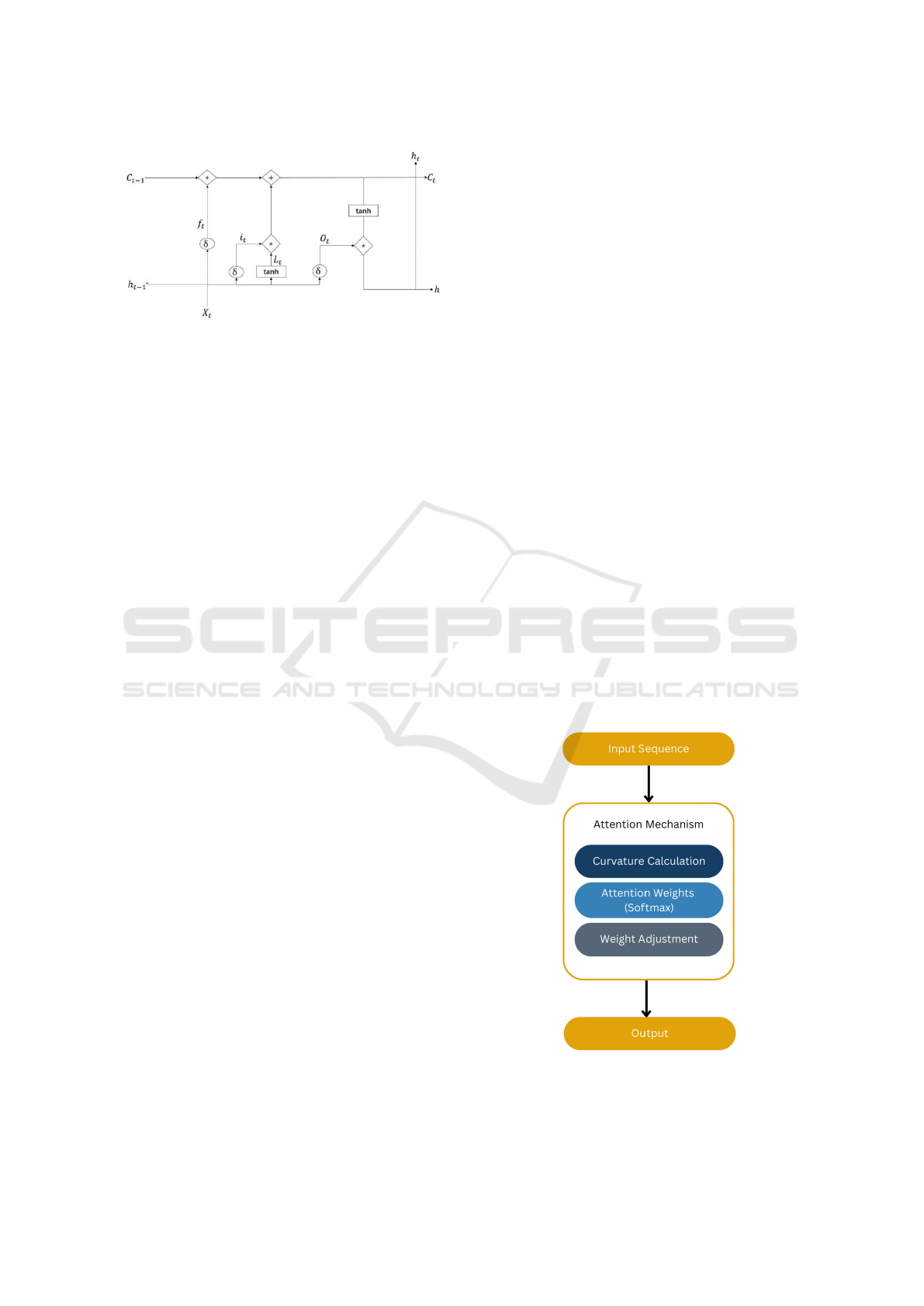
Figure 1: Long Short-Term Memory Network Architecture.

the Update Gate, responsible for time step Zt updates

at time t, and the Reset Gate, determining the extent

to which past information should be discarded in the

current time step. This nuanced architecture provides

an alternative perspective for optimizing time series

forecasting models.

For non-stationary multivariate time series fore-

casting. (Liu and Chen, 2019) introduced a linear

hybrid gate unit, MIXGU, by combining GRU and

MGU models, leading to a synergistic enhancement

of prediction outcomes. Another noteworthy example

is the work of Dai (Dai et al., 2020), who enhanced

PM2.5 concentration prediction in Beijing by inte-

grating the empirical modal decomposition algorithm

(EMD) with LSTM. This hybrid approach surpassed

the predictive accuracy achieved by individual algo-

rithms, emphasizing the importance of tailored adap-

tations for improved forecasting performance.

2 CURVATURE-INFORMED

ATTENTION MECHANISM

FOR LSTM

Time series data typically consists of pairs of val-

ues associated with speciﬁc time periods or points in

time. These pairs comprise two distinct elements: the

temporal component and the numerical value. The

temporal element signiﬁes a particular time period or

point in time, while the numerical element may corre-

spond to a single variable or multiple variables. When

the numerical element pertains to one variable, it is

termed a univariate time series. Conversely, when it

involves multiple variables, it is referred to as a mul-

tivariate time series.

2.1 Long Short-Term Memory Network

The LSTM (Gers, 2002) unit, illustrated in Figure1

involves several components, each serving a distinct

purpose in processing sequential data. Let X

be the

input sequence at time t, h

be the hidden state (mem-

ory), and C

be the cell state. The LSTM components

are deﬁned as follows: The forget gate, denoted as f

decides what information from the cell state should

be discarded. It takes the concatenation of the input

and the previous hidden state h

t−1

as input and out-

puts values between 0 and 1 for each element in the

cell state. The forget gate is deﬁned as follows:

= σ(W

· [h

t−1

, X

] + b

) (1)

where W

is the weight matrix, b

is the bias, and σ is

the sigmoid activation function.

The input gate, denoted as i

, updates the cell state

with new information. Similar to the forget gate, it

takes the concatenation of [h

t−1

, X

] and outputs val-

ues between 0 and 1. The input gate is deﬁned as

follows:

= σ(W

· [h

t−1

, X

] + b

) (2)

The cell state is updated using the forget gate, in-

put gate, and a new candidate value

. The candidate

value

is calculated using the tanh activation func-

tion:

= tanh(W

· [h

t−1

, X

] + b

) (3)

The updated cell state C

is given by:

= f

·C

t−1

+ i

(4)

In these equations, W

, b

, W

, b

, W

, b

, W

, b

represent the weight matrices and biases. The sig-

moid function σ and the hyperbolic tangent function

tanh are used for activation.

Figure 2: The Curvature-Informed Attention Mechanism.

ICAART 2024 - 16th International Conference on Agents and Artiﬁcial Intelligence

1264

2.2 Curvature-Informed Attention

Mechanism CIAM

Attention mechanisms (Ashish et al., 2017) enhance

the capabilities of deep learning models in tasks in-

volving sequential data, such as Natural Language

Processing (NLP) and time series forecasting. The

core idea behind attention is to enable the model to

focus selectively on speciﬁc segments of the input

sequence, assigning varying levels of signiﬁcance to

different elements.

The Curvature-Informed Attention Mechanism

(CIAM) introduces a novel approach by incorporat-

ing the intrinsic curvature measure of the original time

series data, providing a quantiﬁable representation of

variations and trends. The curvature has been em-

ployed in many approaches to recognize and charec-

trize curves (Ayachi et al., 2023) (Ayachi et al., 2020)

(Abbasi et al., 2000). Unlike traditional attention

mechanisms that rely solely on sequential patterns or

external features, CIAM leverages the inherent cur-

vature measure. Figure 2 present an overview of the

approach.

Step 1: Curvature Calculation

The curvature (κ

) for each data point (X

) is computed

by taking the second derivative of the data with re-

spect to time:

(5)

Step 2: Attention Weights Calculation

Attention weights (α

) are determined based on the

softmax function applied to the curvature measures:

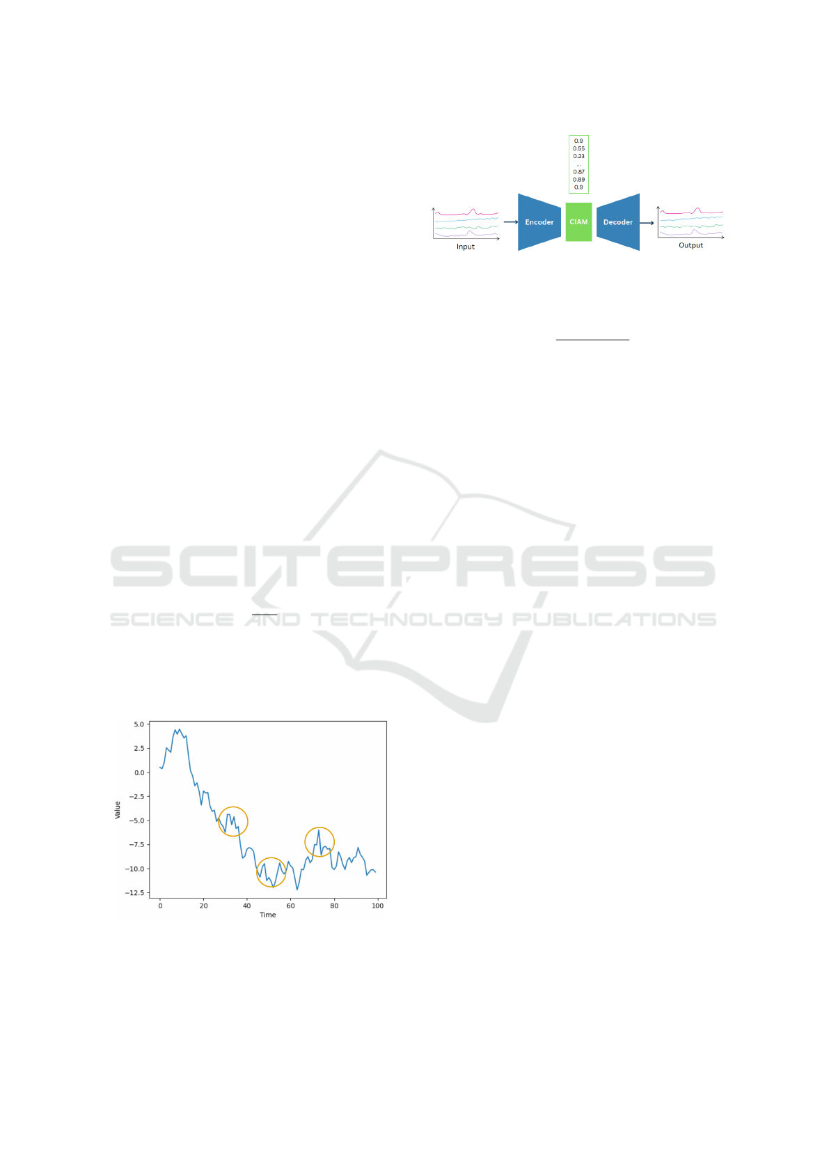
Figure 3: In Blue, a random time serie. In Orange, zones to

be focused on by CIAM. Larger weights are expected to be

attributed to these areas.

Figure 4: CIAM based encoder-decoder architecture. The

input is formed by univariate or multivariate time series.

The output represent the reconstructed initial series.

exp(κ

)

∑

j=1

exp(κ

)

(6)

Step 3: Dynamic Weight Adjustment

Attention weights (α

) are dynamically adjusted to

incorporate curvature values and previous attention

weights, controlled by a hyperparameter (β):

= β · α

+ (1 − β) · κ

(7)

Step 4: Full CIAM Process

The complete CIAM process is expressed as a set of

adjusted attention weights for each data point:

CIAM(X

, X

, . . . , X

) = {α

, α

, . . . , α

} (8)

2.3 Encoder-Decoder Network

The concept of the code-and-decode model

(Sutskever et al., 2014) (Bahdanau et al., 2014)

(Liu et al., 2019) (Junczys-Dowmunt et al., 2018)

initially emerged as a solution for tackling the

seq2seq problem, primarily designed for tasks like

text translation or responding to input queries. As

its application expanded to include time series

prediction, promising results were observed. Despite

its effectiveness over standalone models, the encoder-

decoder model is not without limitations. Its reliance

on a single link between the encoder and decoder,

embodied by a ﬁxed-length vector, poses challenges,

particularly for lengthy input sequences. The ﬁxed-

length vector struggles to retain information from

earlier inputs when processing subsequent ones. To

address this limitation, the attention mechanism has

been integrated into the encoder-decoder model,

aiming to enhance its capacity to capture and utilize

information from the entire sequence.

Within the Curvature-Informed Attention Mecha-

nism (CIAM), the weights undergo dynamic adjust-

ments contingent on the curvature measure of the

original time series data, as illustrated in Figure 3

Curvature-Informed Attention Mechanism for Long Short-Term Memory Networks

1265

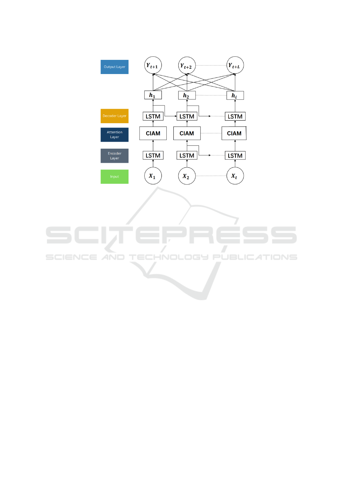
Figure 5: A detailed overview of the CIAM based architecture : The encoding is performed using LSTM, followed by an

attention mechanism based on curvature. The decoding is realized based on an inverse operation to obtain the initial series.

The invertibility characteristic of the curvature enhances the decoding process.

and Figure 4. This entails calculating curvature mea-

sures for each data point, encapsulating variations and

trends in the sequence. The application of the soft-

max function to these curvature values yields atten-

tion weights. Consequently, the attention mechanism

contributes to reﬁning forecasting outcomes, particu-

larly in scenarios characterized by random trends and

seasonality.

The proposed architecture is a robust sequence-to-

sequence model comprising an LSTM-based encoder,

a Curvature-Informed Attention Mechanism (CIAM),

and a decoder LSTM (Figure 5). The LSTM encoder

captures temporal dependencies, while CIAM dy-

namically adjusts attention based on curvature mea-

sures, enabling the model to prioritize signiﬁcant

points in the sequence. The decoder LSTM recon-

structs the time series using information from the en-

coder and CIAM, resulting in an effective and adap-

tive model for accurate time series prediction.

It is noteworthy that the information encoded in

the curvature measure holds the potential for recon-

structing the initial time series curve. This intrinsic

capability adds value to the encoder-decoder archi-

tecture, where the decoder plays a crucial role in the

reconstruction of data.

3 EXPERIMENTATIONS

This section contains a presentation of the evaluation

metrics and used datasets. Subsequently, we delineate

the dataset preprocessing methodology and expound

on the pertinent parameter conﬁgurations for the ex-

periments. The subsequent segment involves an in-

depth analysis and assessment of the experimentally

obtained results.

3.1 Datasets

Our experimentation involved the utilization of ﬁve

publicly accessible datasets: the Beijing Air Qual-

ity dataset (Air)(27, ), the Household Electricity

Consumption dataset from Paris, France (Electric-

ity) (28, ), the Daily Stock dataset (Stock) (29, ),

the Daily Gold Price dataset (Gold) (30, ), and the

Chengdu PM2.5 Concentration dataset (CDPM2.5)

(ByoungSeon, 2012).

The Air dataset originates from the US Embassy

in Beijing, collecting weather and air pollution in-

dices over ﬁve years (2010 to 2014) with hourly gran-

ularity. This multivariate time series dataset encom-

passes variables like time, PM2.5 concentration, dew

point, temperature, atmospheric pressure, wind direc-

tion, wind speed, cumulative hourly snowfall, and cu-

mulative hourly rainfall.

The Electricity dataset, also multivariate, captures

household electricity consumption in Paris from De-

ICAART 2024 - 16th International Conference on Agents and Artiﬁcial Intelligence

1266

Table 1: Overview of Dataset Characteristics for Experi-

mental Evaluation.

Dataset Size Variables

Air 8760 8

Electricity 6120 7

Stock 2426 6

Gold 2227 6

CDPM2.5 8760 9

cember 2006 to November 2010 at one-minute inter-

vals. It includes time, active power per minute, reac-

tive power per minute, average voltage per minute,

average current intensity per minute, and speciﬁc

electricity usage details.

The Stock dataset documents daily stock move-

ments from April 26, 2010, to April 24, 2020, with

daily data points. It incorporates information such as

stock opening price, closing price, all-day high, all-

day low, total, and code.

The Gold dataset records daily gold prices from

January 1, 2014, to August 5, 2022, with daily collec-

tion intervals. It includes data like the daily closing

price of gold, opening price, highest price for the day,

lowest price for the day, total number of trades for the

day, and daily rise and fall.

The ﬁfth dataset pertains to PM2.5 data for

Chengdu from 2010 to 2015, recorded on a daily ba-

sis. Variables cover PM2.5 concentration, dew point

temperature, humidity, pressure, combined wind di-

rection, cumulative wind speed, precipitation, and cu-

mulative precipitation.

3.2 Data Pre-Processing

In the initial data processing stage, we transformed

all ﬁve datasets into a 3D tensor of [sample, time step,

feature], making their format adequate for subsequent

model input. To handle outliers and missing values,

mean ﬁlling was employed for the latter, while the

former were directly removed.

Speciﬁcally, in the case of the AIR dataset, the

non-predictive variable of wind direction was ex-

cluded, and missing values were addressed using

mean ﬁlling. Likewise, the ELECTRICITY dataset

saw the removal of non-compliant variables related

to kitchen active energy, electric water heater, and

air conditioner, with mean ﬁll applied for any miss-

ing values. For the STOCK dataset, non-compliant

coded variables were eliminated. The GOLD dataset

underwent a similar process, removing variables that

didn’t align with experimental requirements. In the

CDPM2.5 dataset, anomalous variables like PM2.5

and combined wind data were excluded, and irrele-

vant variables like precipitation and cumulative pre-

cipitation were also removed. This resulted in ﬁnal

datasets containing 7, 5, 5, 5, and 5 variables, respec-

tively.

During experimentation, datasets were divided

into training and testing sets. For AIR and CDPM2.5,

the ﬁrst 11 months were designated for training, with

the remaining month for testing. Predictors included

wind speed for AIR and humidity for CDPM2.5.

In the ELECTRICITY dataset, the ﬁrst 6000 entries

constituted the training set, and average voltage per

minute was chosen as the ﬁnal predictor. For STOCK,

2376 entries were utilized for training, with the clos-

ing price as the predictor variable. In the GOLD

dataset, the ﬁrst 2160 entries served as the training

set, and the closing price was selected as the predic-

tor variable. Following dataset slicing, a maximum-

minimum normalization process was applied to pre-

vent data discrepancies from affecting results. In the

ﬁnal prediction phase, back-normalization of the data

to its original values was carried out.

3.3 Experimental Parameters

Concerning the experimental conﬁguration, the setup

for each of the ﬁve datasets varied due to differ-

ences in their acquisition intervals. This discrep-

ancy primarily manifested in the time step conﬁgura-

tions. Given the hourly acquisition period of the AIR

dataset, the time step for both AIR and CDPM2.5 was

set to 24, aligning with the predicted length. Sim-

ilarly, for the ELECTRICITY dataset with a collec-

tion period of 1 minute, the time step was conﬁgured

at 30, matching the predicted length. In the cases of

STOCK and GOLD, both with a daily collection pe-

riod, the time step was set to 24, again corresponding

to the predicted length.

As for the model parameters, a consistent epoch

count of 50, a batch size of 128, and a hidden layer

of 100 in the LSTM were employed across all ex-

periments. The activation function utilized was the

ReLU function. To mitigate overﬁtting, a dropout

function was incorporated after each LSTM model,

with a dropout parameter of 0.3. Batch normaliza-

tion was applied to the data to enhance the stability

of the entire neural network at each layer’s intermedi-

ate output. Throughout the training process, the mean

squared error (mse) loss function was chosen, and op-

timization utilized the Adam algorithm with a learn-

ing rate set to 0.001. Additionally, the learning rate

decayed by 1e-5 per round.

Here is a table summarizing the experimental pa-

rameters:

Curvature-Informed Attention Mechanism for Long Short-Term Memory Networks

1267

Table 2: Multivariate time series forecasting results for ﬁve datasets.

Methods

CNN

RMSE MAPE

CNN-LSTM

LSTM

RMSE MAPE

Stacked-LSTM

RMSE MAPE

BiLSTM

RMSE MAPE

Encoder-decoder-LSTM

RMSE MAPE

CIAM LSTM

RMSE MAPE

AIR 1.282 49.85% 1.234 50.09% 1.264 52.17% 1.291 52.74% 1.530 61.83% 1.315 58.86% 1.144 48.42%

ELECTRICITY 2.792 9.54% 0.749 2.68% 0.937 3.31% 1.484 5.15% 1.675 5.79% 0.907 3.21% 0.635 1.53%

STOCK 0.305 60.30% 0.030 12.28% 0.128 30.07% 0.334 61.64% 0.139 29.56% 0.470 79.52% 0.034 11.20%

GOLD 4.878 77.47% 0.507 26.93% 1.506 54.17% 3.205 63.90% 1.238 46.19% 0.690 38.65% 0.203 19.56%

CDPM2.5 0.233 11.52% 0.219 11.11% 0.178 9.03% 0.349 17.72% 0.551 27.62% 0.170 8.39% 0.166 8.01%

Table 3: Experimental Parameters.

Parameter Value

Epoch 50

Batch Size 128

Hidden Layer in LSTM 100

Activation Function ReLU

Dropout Parameter 0.3

Learning Rate 0.001

Learning Rate Decay 1e-5

3.4 Results and Discussion

The comprehensive evaluation of various forecasting

methods on ﬁve distinct datasets, namely AIR, ELEC-

TRICITY, STOCK, GOLD, and CDPM2.5, is pre-

sented in Table 2. The performance metrics, includ-

ing root mean square error (RMSE) and mean abso-

lute percentage error (MAPE), provide insights into

the effectiveness of each method.

For the AIR dataset, the CIAM LSTM outper-

forms other models, achieving an RMSE of 1.144 and

a MAPE of 48.42%. Notably, it surpasses baseline

models such as CNN, CNN-LSTM, LSTM, Stacked-

LSTM, BiLSTM, and Encoder-decoder-LSTM in

both metrics.

In the case of ELECTRICITY, CIAM LSTM

demonstrates superior performance with an RMSE of

0.635 and a MAPE of 1.53%, outclassing alternative

methods like CNN, CNN-LSTM, LSTM, Stacked-

LSTM, BiLSTM, and Encoder-decoder-LSTM.

For the STOCK dataset, CIAM LSTM excels with

an RMSE of 0.034 and a MAPE of 11.20%, showcas-

ing its effectiveness compared to competing models.

In the GOLD dataset, CIAM LSTM again exhibits

strong performance, achieving an RMSE of 0.203 and

a MAPE of 19.56%, surpassing several other meth-

ods.

For the CDPM2.5 dataset, CIAM LSTM demon-

strates competitive accuracy, with an RMSE of 0.166

and a MAPE of 8.01%, showcasing its efﬁcacy in

multivariate time series forecasting.

Overall, the results highlight the robustness of

the proposed CIAM LSTM, consistently providing

accurate predictions across diverse datasets. These

ﬁndings emphasize the potential of the Curvature-

Informed Attention Mechanism in enhancing LSTM-

based forecasting models for various multivariate

time series applications.

4 CONCLUSION

In conclusion, the Curvature-Informed Attention

Mechanism (CIAM) stands out as an explainable

and interpretable enhancement to traditional attention

mechanisms in the realm of time series forecasting.

By incorporating the intrinsic curvature measures of

the original time series data, CIAM introduces a novel

approach that surpasses conventional methods relying

solely on sequential patterns or external features.

The dynamic adjustment of attention weights, in

an encoder-decoder architecture, based on curvature

measures empowers CIAM to discern and prioritize

the signiﬁcance of various points within a sequence.

This adaptability is particularly valuable in scenar-

ios characterized by random trends, where patterns

defy regular trajectories. Unlike rigid attention mech-

anisms that may struggle to capture unpredictable

variations, CIAM focuses on dynamically allocating

attention, enabling the model to ﬂexibly respond to

important deviations and nuanced ﬂuctuations in the

data.

The experimental results, as showcased in the

presented multivariate time series forecasting results

for ﬁve diverse datasets, demonstrate the efﬁcacy of

CIAM. Notably, CIAM exhibits superior performance

in comparison to established methods like CNN,

LSTM, and Encoder-decoder-LSTM across various

evaluation metrics such as RMSE and MAPE. This re-

inforces the notion that incorporating curvature mea-

sures in the attention mechanism signiﬁcantly con-

tributes to the model’s predictive accuracy, especially

in the presence of random trends and intricate season-

ality patterns.

The invertibility characteristic of the curvature

makes it a promising foundation for an encoder-

decoder model. Mainly in the decoding part where

the reconstruction process utilizes the this character-

istic to rebuild the original time serie.

In summary, CIAM not only advances the current

state-of-the-art in time series forecasting but also pro-

vides a conceptual framework for integrating intrinsic

ICAART 2024 - 16th International Conference on Agents and Artiﬁcial Intelligence

1268

data characteristics into attention mechanisms. This

novel approach represents a step forward in enhancing

the predictive capabilities of machine learning mod-

els, laying the foundation for more sophisticated and

adaptive forecasting methodologies.

REFERENCES

(apr. 5, 2022). beijing pm2.5 dataset.

[online]. available: https://

archive.ics.uci.edu/ml/datasets/beijing+pm2.5+data.

(apr. 5, 2022). daily gold price dataset. [online]. available:

https://www.kaggle.com/datasets/nisargchodavadiya/

daily-gold-price20152021-time-serie.

(apr. 5, 2022). daily stock dataset. [online]. available:

https://www.kaggle.com/datasets/dsadads/databases.

(apr. 5, 2022). individual household electric power

consumption dataset. [online]. available:

https://archive.ics.uci.edu/ml/datasets/ individ-

ual+household+electric+power+consumption.

Abbasi, S., Mokhtarian, F., and Kittler, J. (2000). Enhanc-

ing css-based shape retrieval for objects with shallow

concavities. Image and vision computing, 18(3):199–

211.

Ashish, V., Shazeer, N., Parmar, N., Uszkoreit, J., Jones, L.,

Gomez, A. N., Kaiser,

A., and Polosukhin, I. (2017).

Attention is all you need. In Proc. Adv. Neural Inf.

Process. Syst., volume 30, pages 105–109.

Ayachi, L., Benkhlifa, A., Jribi, M., and Ghorbel, F. (2020).

Une nouvelle description du contour de l’espace: Une

repr

esentation espace-echelle g

eralis

ee bas

ee sur la

courbure et la torsion.

Ayachi, L., Jribi, M., and Ghorbel, F. (2023). General-

ized torsion-curvature scale space descriptor for 3-

dimensional curves.

Bahdanau, D., Cho, K., and Bengio, Y. (2014). Neural ma-

chine translation by jointly learning to align and trans-

late. arXiv preprint arXiv:1409.0473.

Box, G. (2015). Time Series Analysis: Forecasting and

Control. Wiley, San Francisco, CA, USA.

ByoungSeon, C. (2012). ARMA Model Identiﬁcation.

Springer, New York, NY, USA.

Cho, K., van Merrienboer, B., Bahdanau, D., and Bengio,

Y. (2014). On the properties of neural machine trans-

lation: Encoder-decoder approaches.

Dai, S., Chen, Q., Liu, Z., and Dai, H. (2020). Time se-

ries prediction based on emd-lstm model. J. Shenzhen

Univ. Sci. Eng., 37(3):221–230.

Gers, F. (2002). Applying lstm to time series pre-

dictable through time-window approaches. In Neural

Nets WIRN Vietri-01, pages 193–200, London, U.K.

Springer.

Junczys-Dowmunt, M., Grundkiewicz, R., Dwojak, T.,

Hoang, H., Heaﬁeld, K., Neckermann, T., Seide, F.,

Wiesler, S., Germann, U., and Fikri Aji, A. (2018).

Marian: Fast neural machine translation in c++. arXiv

preprint arXiv:1806.09235.

Liu, J. and Chen, S. (2019). Non-stationary multivariate

time series prediction with mix gated unit. J. Comput.

Res. Develop., 56(8):1642.

Liu, Y., Ott, M., Goyal, N., Du, J., Joshi, M., Chen,

D., Levy, O., Lewis, M., Zettlemoyer, L., and Stoy-

anov, V. (2019). Bert: Pre-training of deep bidirec-

tional transformers for language understanding. arXiv

preprint arXiv:1810.04805.

McLeod, A. I. and Li, W. K. (1983). Diagnostic check-

ing arma time series models using squared-residual

autocorrelations. Journal of Time Series Analysis,

4(4):269–273.

Nakkach, C., Zrelli, A., and Ezzeddine, T. (2022). Deep

learning algorithms enabling event detection: A re-

view. In 2nd International Conference on Industry

4.0 and Artiﬁcial Intelligence (ICIAI 2021). Atlantis

Press.

Nakkach, C., Zrelli, A., and Ezzedine, T. (2023). Long-term

energy forecasting system based on lstm and deep ex-

treme machine learning. Intelligent Automation & Soft

Computing, 37(1).

Sutskever, I., Vinyals, O., and Le, Q. V. (2014). Sequence

to sequence learning with neural networks. Advances

in neural information processing systems.

Torres, J. L., Garc

ıa, A., Blas, M. D., and De Francisco,

A. (2005). Forecast of hourly average wind speed

with arma models in navarre (spain). Solar Energy,

79(1):65–77.

Yu, Y., Si, X., Hu, C., and Zhang, J. (2019). A review of

recurrent neural networks: Lstm cells and network ar-

chitectures. Neural Computation, 31(7):1235–1270.

Curvature-Informed Attention Mechanism for Long Short-Term Memory Networks

1269