Discrimination of Signals from Large Covariance Matrix for Pattern

Recognition

Masaaki Ida

National Institution for Academic Degrees and Quality Assurance of Higher Education, Kodaira, Tokyo, Japan

Keywords: Pattern Recognition, Eigenvalue Distribution, Signal, Randomness, Large Covariance Matrix, Neural Network.

Abstract: Pattern recognition applications and methods are important areas in modern data science. One of the

conventional issues for the analysis is the selection of important signal eigenvalues from many eigenvalues

dominated by randomness. However, appropriate theoretical reason for selection criteria is not indicated. In

this paper, investigating eigenvalue distribution of large covariance matrix for data matrix, comprehensive

discrimination method of signal eigenvalues from the bulk of eigenvalues due to randomness is investigated.

Applying the discrimination method to weight matrix of three-layered neural network, the method is examined

by handwritten character recognition example.

1 INTRODUCTION

Data Science is rapidly spreading particularly in

business and social science fields such as psychology

or education. In various data analysis methods, the

eigenvalues and eigenvalue distributions of variance-

covariance matrices or correlation matrices are often

studied. The issue is identifying whether the

eigenvalue is an important one or not. In other word,

signal eigenvalue selection is the problem that is

encountered in various data analysis situations.

As conventional selection methods,

predetermined number of selected eigenvalues (two,

three and so on) is adopted as selection criteria, or

predetermined cumulative contribution ratio of

eigenvalues (e.g., 50% or 70-80% and so on) is

sometimes adopted as selection criteria. However, the

criteria depends on the analysis situation, and there is

no appropriate theoretical reason as selection criteria.

Another powerful selection or discrimination

method uses random matrix theory. This method

examines the difference between the eigenvalue

distribution of sample covariance matrices of large

random data matrix and the distribution of real data

matrix including randomness and signal features.

However, all eigenvalues included in the difference

do not have important signal properties.

https://orcid.org/0009-0004-4681-6811

In this (work in progress) research based on the

idea of random matrix theory, discrimination method

of important signal eigenvalues from the bulk of

random eigenvalues is discussed.

In order to consider the feature of eigenvalues, by

performing singular value decomposition of the data

matrix, then data matrix is reconstructed by

combining the important singular values. By

performing statistical hypothesis test on the

reconstructed matrix, we obtain information that

identifies whether the eigenvalues are important or

not.

The contents of this paper are summarized as

follows: (i) investigate the eigenvalue distribution

that can be separated to the random part and the signal

part of eigenvalues, and explain discrimination

method, (ii) apply the method to weight matrix of

three-layered artificial neural network for simple

MNIST dataset as a pattern recognition application.

The discrimination method is explained by showing

numerical example.

2 EIGENVALUE DISTRIBUTION

Data models mainly dominated by randomness have

been frequently studied in Random Matrix Theory

(Bai 2010, Couillet 2011, Couillet 2022). In this

866

Ida, M.

Discrimination of Signals from Large Covariance Matrix for Pattern Recognition.

DOI: 10.5220/0012463300003654

Paper published under CC license (CC BY-NC-ND 4.0)

In Proceedings of the 13th International Conference on Pattern Recognition Applications and Methods (ICPRAM 2024), pages 866-871

ISBN: 978-989-758-684-2; ISSN: 2184-4313

section, we see the results of random matrix theory

related to eigenvalue distribution.

The formulation of this paper is as C = X

X / n,

where X is an n x p random data matrix. Eigenvalues

of the matrix C are denoted λ

(k = 1, ..., p) with

ranking in descending order. Based on Random

Matrix Theory, asymptotic eigenvalue distribution

can be calculated with enlarging the matrix size to

infinity.

In general, eigenvalue distribution of random data

agrees with the predicted eigenvalue distribution

based on Random Matrix Theory, which is called

Marchenko-Pastur (MP) distribution. Under the

condition that n, p go to infinity with p/n goes to c,

asymptotic distribution of eigenvalues with random

entries, P(λ), is described as follows:

P(λ) = ((λ

- λ) (λ - λ

))

0.5

/ (2πcλ)

(1)

where λ

= (1 + c

0.5

)

, λ

= (1 - c

0.5

)

. As an

approximation in real case, we can apply it to finite

large covariance matrix.

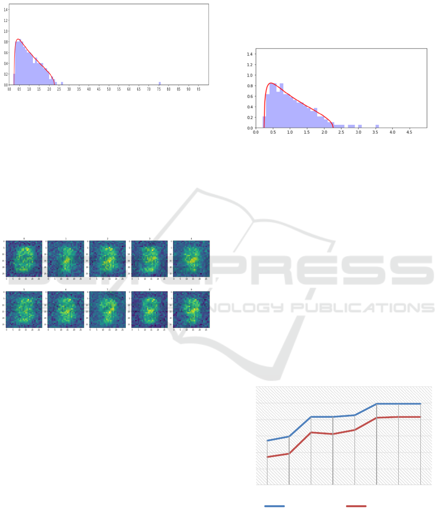
As seen in Figure 1, red curve shows the MP

distribution, which are fit to distribution of random

bulk histogram.

Figure 1: Example of MP distribution. horizontal axis:

eigenvalue, vertical axis: density.

However, many empirical studies indicate that the

eigenvalue distribution of actual data matrix has

dominant random eigenvalues (bulk) and small

number of large eigenvalues (signals or spikes) that

are not random related eigenvalues (Plerou 2002,

Baik 2006). This is shown in Figure 1.

The studies for the phenomena in references

(Martin 2019, Martin 2021) describe that eigenvalues

distributions are classified into some types of

distributions such as Random-like, Bulk-Spikes, Bulk-

Decay, Heavy-tailed, and so on. Figure 1 is an

example of Bulk-Decay-Spikes type distribution with

random bulk in left side and other signal eigenvalues

in right side.

This MP distribution can be used as a method to

distinguish whether eigenvalues have randomness or

signal characteristics. In other words, assume that the

eigenvalues included in the red distribution have

randomness, and the eigenvalues on the right which

are not included in the MP distribution have signal

characteristics.

However, in actual eigenvalue distribution, the

boundary or separation point between random part

and signal part is not necessarily clear. Therefore,

appropriate discrimination or extraction method of

signals from eigenvalue distribution is important.

Other question is whether all eigenvalues that deviate

to the right from the red MP distribution are signals

or not. It is true that properties other than randomness

are included in such eigenvalues, but not all of them

necessarily have important meaning.

Regarding this issue, the author's past initial

experiments have confirmed that there are cases in

which the separation based on the MP distribution

and the separation suggested by statistical tests almost

match. However, in general, this may not always be

the case. In this paper, we will deeply consider this

issue.

3 DISCRIMINATION METHOD

In this paper, signal discrimination method is

extended which is based on the eigenvalue

distribution of random matrix theory but does not

simply depend on the MP distribution. Particularly

focusing on Bulk-Spikes or Bulk-Decay type

distribution, discrimination method of signals from

eigenvalue distribution of large covariance matrix is

investigated.

First, we perform singular value decomposition of

the data matrix. Next, we consider the method for

identifying signals by reconstructing data matrix

using the important singular values and performing

the statistical test on the matrix. The final signal

discrimination is determined comprehensively by

combining the indication of statistical test and other

considerations. This method provides an appropriate

indication of separation point for signal eigenvalues.

Data matrix reconstruction in the above process

means ‘Sparsification’ which extracts and utilizes

only useful eigenvalues.

[Discrimination method]

Set: Target data matrix X.

Process: Singular value decomposition for the

target data matrix, X = U diag(s) V

, where s is a

list of singular values (descending order), ‘diag’

means a diagonal matrix, U is a matrix of left-

singular vectors, and V is a matrix of right-

singular vectors.

while not appropriate separation do

Discrimination of Signals from Large Covariance Matrix for Pattern Recognition

867

Set: sp (separation point) = minimum singular

value (eigenvalue) of candidate signals.

Set: Reconstruction matrix X’ = U diag(s’) V

where s’ is a list of singular values of 1 to sp

from s.

Process: Hypothesis test (Kolmogorov–

Smirnov test for normality) for X’.

Check p-value and average p-values for

columns and rows of (standardized) X’.

if p-values of the test < 0.05 then

determine the distribution is not normally

distributed.

Addition of new singular value to

candidate signals.

Go to next section.

else

Subtraction of singular value from

candidate signals.

Go to next section.

end

Algorithm 1: Discrimination process.

The final signal discrimination is determined

comprehensively by combining the indication of

Algorithm 1 and the following considerations:

 Consider the eigenvalue distribution of the MP

distribution.

 Consider real-world applications of hypothesis

testing for normality.

 In the case of supervised learning, consider the

relationship with the accuracy or correct

recognition rate.

4 APPLICATIONS

4.1 Pattern Recognition Application

In this paper, as an application of the discrimination

method, weight matrices of artificial neural network

are examined. The network structure is restricted to

the simple three-layered structure with random data

entries as initial data. This basic experimental

structure has been frequently studied in machine

learning field. The network consists of input layer,

intermediate layer (hidden layer) and output layer.

The network weight matrices are dented W

(from input layer to hidden layer) and W

(from

hidden layer to output layer). The activation function

of each node is the sigmoid function. The weight

update of network connection is based on the

conventional backpropagation rule. In this section we

examine the weight matrix W

(from input layer to

hidden layer) as the target data matrix X described in

previous section.

[Target data]

A concrete target data of this experiments is

commonly used MNIST dataset, which is the dataset

of ten types of handwritten number images and

consists of 784 elements (28 x 28 grayscale image)

associated with labels of ten classes as shown in

Figure 2

Figure 2: Ten classes of MNIST images.

As numerical examples, number of training (test)

data is 200 (100) randomly selected from 60000

(10000) MNIST dataset. The networks’ hidden nodes

= 200, and learning rate = 0.1.

The author's past initial experiments have

confirmed that there are cases in which the separation

based on the MP distribution and the separation

suggested by statistical tests almost match. However,

various other cases were not considered. In the case

of this MNIST, many eigenvalues occur outside the

MP distribution. In this paper, we will deeply

consider this issue.

It should be noted that the following figures are

one trial of experiments. Since the learning process is

stochastic, result might change to some extent in each

experiment.

4.2 Initial Learning Stage

In initial stage (epoch = 1) of learning process,

average of accuracy or correct recognition rate is 0.55

(std:0.09 for 100 trials) for training data, and about

0.4 for test data. Since it is an early stage of learning,

learning is biased strongly depending on the training

data. Therefore, we perform the same initial training

100 times and show the average and standard

deviation of the correct recognition rate.

The eigenvalue distribution of network weight

is shown in Figure 3. The horizontal axis means

eigenvalue and vertical axis is its density. The blue

histogram corresponds eigenvalues of covariance of

data matrix W

In this figure, the distinctive random bulk (blue

bulk) is recognized in the left side of the figure, and a

small number of signal eigenvalues are recognized in

the right side of the figure (e.g., around 7 or 3 in this

case). Therefore, The figure shows an eigenvalue

distribution which can be regarded as a typical Bulk-

ICPRAM 2024 - 13th International Conference on Pattern Recognition Applications and Methods

868

Spikes type of eigenvalue distribution. This is the case

when there are a few eigenvalues that fall outside the

MP distribution.

Figure 3: The eigenvalue distribution of network weight

of initial stage of learning process.

In order to consider the state of learning process,

back query is performed. Back query is the inverse

query from output layer with fixed class vale for

corresponding ten classes to input layer (28 x 28

image layer).

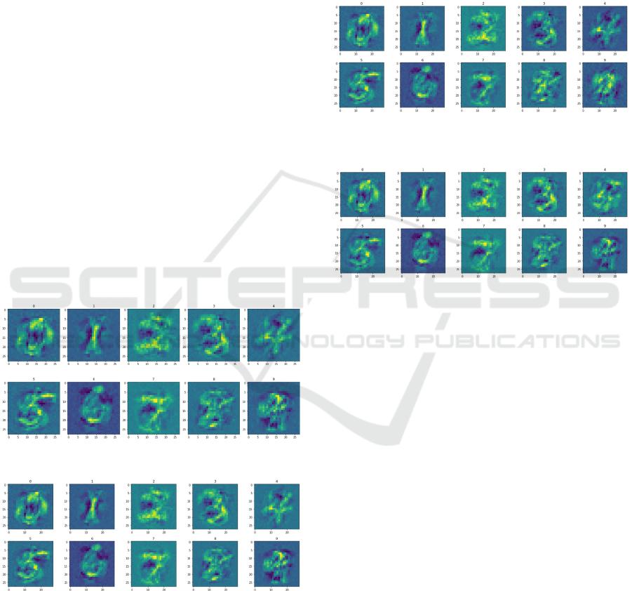
Figure 4 shows back query images of initial

learning stage, which is the blurred images of back

query from output layer to input layer. This figure

shows undifferentiated initial learning stage.

Figure 4: Back query images of initial learning stage.

4.3 Late Learning Stage

4.3.1 Eigenvalue Distribution

Late learning stage (epoch = 50 or 100): Correct

recognition rate for the test data is about 1.0 for

training data and about 0.8 for test data. The

eigenvalue distribution of network weight W

shown in Figure 5. There are many other eigenvalues

outside the right side of this figure (73, 63, 59, 55, 50,

… ).

In this figure, the distinctive random bulk (blue

bulk) is recognized in the left side of the figure, and

many signal eigenvalues are recognized in the right

side of the figure and outside the figure. There are

many (more than 15) eigenvalues that located outside

the MP distribution.

Unlike conventional identification methods,

where eigenvalues that are located outside the MP

distribution are important, it is necessary to select

eigenvalues that have influence on the recognition

rate. Therefore, careful selecting and extracting is

needed. It is difficult to separate between the left

random bulk and right signal values. Therefore, for

searching the appropriate separation, proposed

discrimination method is applied.

Figure 5: Eigen value distribution in late learning stage.

4.3.2 Application of Discrimination Method

For standardized reconstructed weight matrix without

first to sixth (6th) eigenvalues, the KS test indicates

the hypothesis that the distribution of the element is

‘normal distribution’ is rejected. On the other hand,

For standardized reconstructed weight matrix without

first to seventh (7th) eigenvalues, the KS test

indicates the hypothesis that the distribution of the

element is ‘normal distribution’ is not rejected.

In other words, by the KS test, the 6th to 7th

eigenvalues are candidates for eigenvalue separation.

Figure 6 shows blue line as accuracy for training

data of 50 epoch. Green line shows for test data of 50

epochs. This figure indicates that at the nineth and

tenth eigenvalue, correct recognition rates is saturated.

Since the KS test is a hypothesis test, if we allow a

little margin, we can say that the 9th and 10th

eigenvalues are actually reasonable separation points.

Figure 6: Accuracy for reconstructed matrix.

0,2

0,4

0,6

0,8

1,2

56789101112

CR-Re50-training CR-Re50-test

Discrimination of Signals from Large Covariance Matrix for Pattern Recognition

869

4.3.3 Accuracy of Reconstructed Weight

Matrix

Reconstructed weight matrix using the 1st to nth

eigenvalues is examined. As seen in figure 6, in case

of n>=10, the accuracy rate is approximately 1.0 for

the training data and approximately 0.8 for the test

data. In other words, it can be seen that only a limited

number of "signal eigenvalues" are sufficient for the

pattern recognition.

Furthermore, it can be seen even in the case of

n=7 that accuracy rates of 0.8 or higher and 0.6 or

higher are recognized for the reconstructed weight

matrix.

4.3.4 Confirmation by Back Query

Here, back query is considered. As a comparison data,

Figure 7 shows the result images of the back query

from output layer to input layer with original weight

matrix. Figure 8 shows the back query images for the

reconstruction matrix with combination from first

eigenvalue to tenth eigenvalue. These two figures

shows very similar images. In other words, it can be

seen graphically that sufficient approximation is

obtained even with the reconstructed weight matrix.

This means that ‘Sparsification’ is sufficient with the

reconstructed matrix.

Figure 7: Back query images of late learning stage.

Figure 8: Back query images for reconstructed weight

matrix with combination of first eigenvalue to tenth

eigenvalue.

4.3.5 Correspondence Between Eigenvalues

and Images

Correspondence between each eigenvalue and the

identified image is considered.

Figure 9 shows the case of first eigenvalue. This

is the result of back query using the weight matrix of

only the first eigenvalue.

Figure 10 shows some different parts of images

(bright points) that are attracting attention.

Large signal eigenvalues are closely related to

individual classes of digits. The relationship between

eigenvalues and image classes are recognized.

Figure 9: Back query images for the reconstruction with the

first eigenvalue.

Figure 10: Back query images for the reconstruction with

the sixth eigenvalue.

5 CONCLUSIONS

The summary of this paper is as follows: (i)

investigate the eigenvalues that can be separated to

the random part and the signal part of eigenvalues,

and explain discrimination method, (ii) apply the

method to weight matrix of three-layered artificial

neural network, and explain the discrimination

method by showing the example of MNIST dataset.

In this paper, distribution of specific Bulk-Decay-

Spikes type is considered. As for data matrix,

extending the ideas of this paper to the weight matrix

of deep learning networks is expected. The results of

this paper will also lead to the refinement of various

data analysis methods that utilize eigenvalue

distribution including Principal Component Analysis

and other data science methods.

We are currently implementing this discrimination

method on CNN (convolutional neural network) rather

than a simple three-layer neural network. In that case,

the random part also has properties different from the

MP distribution. Therefore, further improvement of the

identification method will be required.

ICPRAM 2024 - 13th International Conference on Pattern Recognition Applications and Methods

870

REFERENCES

Bai, Z. and Silverstein, J. W. (2010) Spectral analysis of

large dimensional random matrices, Springer.

Couillet, R. and Debeeh, M. (2011) Random matrix

methods for wireless communications, Cambridge.

Couillet, R. and Liao, Z. (2022) Random matrix methods

for machine learning, Cambridge.

Baik, J. and Silverstein, J. W. (2006) Eigenvalues of large

sample covariance matrices of spiked population

models, Journal of Multivariate Analysis, 97, pp. 1382-

1408.

Kolmogorov–Smirnov test, Encyclopaedia of Mathematics,

EMS Press, 2001.

Martin, C. H. and Mahoney, M. W. (2019) Traditional and

Heavy-Tailed Self Regularization in Neural Network

Models, https://arxiv.org/abs/1901.08276v1.

Martin, C. H. and Mahoney, M. W. (2021) Implicit self-

regularization in deep neural networks: evidence from

random matrix theory and implications for learning,

Journal of Machine Learning Research, 2021, 22,

1−73.

MNIST, Mixed National Institute of Standards and

Technology database, https://github.com/pjreddie/

mnist-csv-png

Pattern recognition

https://en.wikipedia.org/wiki/Pattern_recognition

Plerou, V. et.al, (2002) Random matrix approach to cross

correlation in financial data, Physical Review, 65,

066126.

Discrimination of Signals from Large Covariance Matrix for Pattern Recognition

871