Depth Estimation Using Weighted-Loss and Transfer Learning

Muhammad Adeel Hafeez

1 a

, Michael G. Madden

1,2 b

, Ganesh Sistu

3 c

and Ihsan Ullah

1,2 d

Machine Learning Research Group, School of Computer Science, University of Galway, Ireland

Insight SFI Research Centre for Data Analytics, University of Galway, Ireland

Valeo Vision Systems, Tuam, Ireland

Keywords:

Depth Estimation, Transfer Learning, Weighted-Loss Function.

Abstract:

Depth estimation from 2D images is a common computer vision task that has applications in many ﬁelds

including autonomous vehicles, scene understanding and robotics. The accuracy of a supervised depth estima-

tion method mainly relies on the chosen loss function, the model architecture, quality of data and performance

metrics. In this study, we propose a simpliﬁed and adaptable approach to improve depth estimation accu-

racy using transfer learning and an optimized loss function. The optimized loss function is a combination of

weighted losses to which enhance robustness and generalization: Mean Absolute Error (MAE), Edge Loss

and Structural Similarity Index (SSIM). We use a grid search and a random search method to ﬁnd optimized

weights for the losses, which leads to an improved model. We explore multiple encoder-decoder-based mod-

els including DenseNet121, DenseNet169, DenseNet201, and EfﬁcientNet for the supervised depth estimation

model on NYU Depth Dataset v2. We observe that the EfﬁcientNet model, pre-trained on ImageNet for classi-

ﬁcation when used as an encoder, with a simple upsampling decoder, gives the best results in terms of RSME,

REL and log

: 0.386, 0.113 and 0.049, respectively. We also perform a qualitative analysis which illustrates

that our model produces depth maps that closely resemble ground truth, even in cases where the ground truth

is ﬂawed. The results indicate signiﬁcant improvements in accuracy and robustness, with EfﬁcientNet being

the most successful architecture.

1 INTRODUCTION

In the context of computer vision, depth estimation

is the task of ﬁnding the distance of different ob-

jects from the camera in an image. The process of

depth estimation has been widely used in many appli-

cation areas including Simultaneous Localization and

Mapping (SLAM) (Alsadik and Karam, 2021), Ob-

ject Recognition and Tracking (Yan et al., 2021), 3D

Scene Reconstruction (Murez et al., 2020), human ac-

tivity analysis (Chen et al., 2013), and more.

Depth estimation can be done with various meth-

ods such as geometry-based methods in which the

depth 3D information of an image is retrieved us-

ing multiple images captured from different positions.

There are also sensor-based methods, which use Li-

DAR, RADAR and ultrasonic sensors for depth esti-

mation. A single camera image can be post-processed

https://orcid.org/0000-0002-3593-7448

https://orcid.org/0000-0002-4443-7285

https://orcid.org/0009-0003-1683-9257

https://orcid.org/0000-0002-7964-5199

by AI-based modalities for depth estimation, by lever-

aging advanced machine learning and computer vi-

sion techniques to estimate depth information from

monocular images (Zhao et al., 2020). Sensor-based

methods have multiple limitations such as hardware

costs and high power requirements relative to camera-

based methods, and are therefore often avoided in

portable and mobile platforms (Sikder et al., 2021).

Although AI-based camera methods are more popular

these days, they also have multiple limitations such as

their computational cost, lack of interpretability and

generalization challenges (Masoumian et al., 2022).

Over the past few years, both unsupervised and su-

pervised methods for depth estimation have become

popular. The unsupervised methods provide better

generalization and reduce data annotation cost (Go-

dard et al., 2017), whereas the supervised learning

methods are more accurate and provide better ex-

plainability, in general, (Patil et al., 2022). Supervised

learning methods are typically characterized by their

simplicity compared to unsupervised methods and the

high degree of adaptability for future modiﬁcations

and enhancements (Alhashim and Wonka, 2018).

780

Hafeez, M., Madden, M., Sistu, G. and Ullah, I.

Depth Estimation Using Weighted-Loss and Transfer Learning.

DOI: 10.5220/0012461300003660

Paper published under CC license (CC BY-NC-ND 4.0)

In Proceedings of the 19th International Joint Conference on Computer Vision, Imaging and Computer Graphics Theory and Applications (VISIGRAPP 2024) - Volume 2: VISAPP, pages

780-787

ISBN: 978-989-758-679-8; ISSN: 2184-4321

The accuracy of supervised methods usually de-

pends upon two factors: 1) the loss function; 2) the

model architecture. Based on the previous studies

and experimental analysis, our goal in this paper is

to propose a method which is simpler, easy to train,

and easy and modify. For this, we mainly rely on

optimizing existing loss functions and using trans-

fer learning. Our experiments show that using high-

performing pre-trained models via transfer learning,

which were originally designed and trained for clas-

siﬁcation along with the optimized loss function can

provide better accuracy, and reduce the root mean

square error (RMSE) for the depth estimation prob-

lems.

Our main contributions are the following:

• We propose an optimized loss function, which can

be used for ﬁnetuning a pre-trained model.

• We perform an exploratory analysis with various

pre-trained models.

• After analysing the ground truth provided with

datasets (NYU Depth Dataset v2), we identiﬁed

some discrepancies in the dataset and how the pro-

posed approach handled them.

• We report the performance compared to the exist-

ing models and loss functions.

While our approach advances the ﬁeld of depth

estimation, we acknowledge certain limitations in

its current form, particularly for safety-critical ap-

plications where traditional image pair methods are

renowned for their reliability (Mauri et al., 2021).

2 LITERATURE REVIEW

In the ﬁeld of depth estimation, various methodolo-

gies have been explored over the years, including both

traditional and deep learning-based approaches. Tra-

ditional depth estimation primarily relied on stereo

vision and structured light techniques. Stereo vi-

sion methods, such as Semi-Global Matching (SGM)

(Hirschmuller and Scharstein, 2008), computed depth

maps by matching corresponding points in stereo im-

age pairs. Structured light approaches used known

patterns projected onto scenes to infer depth (Fu-

rukawa et al., 2017). These methods laid the founda-

tion for depth estimation and remain relevant in spe-

ciﬁc scenarios.

In the past decade, deep learning-based depth esti-

mation methods have made signiﬁcant advancements.

Eigen et al. (2014) introduced an early deep learn-

ing model that used a convolutional neural network

(CNN) to estimate depth from single RGB images.

More recent supervised methods have introduced ad-

vanced architectures such as U-Net (Yang et al., 2021)

and MobileXNet (Dong et al., 2022) for improved

depth prediction.

Unsupervised depth estimation approaches have

also gained prominence, eliminating the need for la-

belled data. Garg et al. (2016) proposed a novel

framework that leveraged monocular stereo supervi-

sion, achieving competitive results without depth an-

notations. Other unsupervised methods use the con-

cept of view synthesis, where images are reprojected

from the estimated depth map to match the input im-

ages. This self-consistency check encourages the net-

work to produce accurate depth maps without explicit

supervision (Godard et al., 2017).

Traditional loss functions play a crucial role in

training depth estimation models. Common loss func-

tions include Mean Squared Error (MSE) (Torralba

and Oliva, 2002) and Mean Absolute Error (MAE)

(Chai and Draxler, 2014), which measure the squared

and absolute differences between predicted and true

depth values, respectively. Additionally, the Hu-

ber loss (Fu et al., 2018) offers a compromise be-

tween MSE and MAE, providing robustness to out-

liers. Huber loss is a hybrid loss function that uses

MSE for small errors and MAE for large errors, mak-

ing it more robust to outliers (Tang et al., 2019).

Other loss functions, such as structural similarity

index (SSIM) (Wang et al., 2004), focus on per-

ceptual quality, promoting visually enhanced depth

maps. These losses have been reported individually

(Carvalho et al., 2018) as well as in the combined

functions, like MAE-SSIM, Edge-Depth, and Huber-

Depth, enhancing the overall accuracy and perceptual

quality of depth predictions (Paul et al., 2022).

3 METHODOLOGY

In this section, we will discuss the dataset we used,

the loss functions, the models, and the training pro-

cess.

3.1 Dataset

In this study, we have used NYU Depth Dataset ver-

sion 2 (Silberman et al., 2012). This dataset com-

prises video sequences from different indoor scenes,

recorded by RGB and Depth cameras (Microsoft

Kinect). The dataset contains 120,000 training im-

ages, with an original resolution of 640 ×480 for both

the RGB and depth maps. In this dataset, the depth

maps have an upper bound limit of 10 meters which

means that any object that is 10 meters or more from

Depth Estimation Using Weighted-Loss and Transfer Learning

781

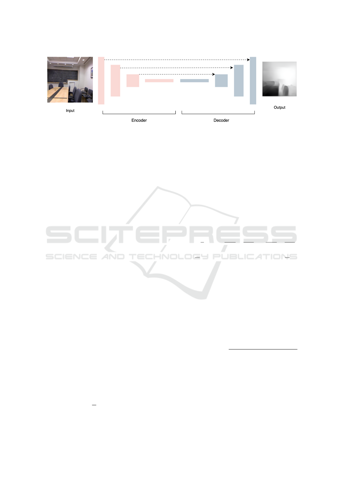
Figure 1: Overview of the network. We implemented a simple encoder-decoder-based network with skip connections. We

changed the encoder between different models while keeping the decoder constant. The depth maps produced at the output

were 1/2X of the ground-truth maps.

the camera will have the maximum depth value. To

reduce the decoder complexity and to save the train-

ing time, we kept the dimensions of the output of

our model (depth maps) to half of the original di-

mensions (320 × 240) and down-sampled the ground

depth to the same dimensions before calculating the

loss as reported previously (Li et al., 2018). The orig-

inal data source contained both RAW (RGB, depth

and accelerometer data) ﬁles and pre-processed data

(missing depth pixels were recovered through post-

processing). We used this processed data and did not

apply any further pre-processing to the data. The test

set contained 654 pairs of original RGB images and

their corresponding depth values.

3.2 Loss Functions

Loss functions play a crucial role while training a

deep learning algorithm. Loss functions help to quan-

tify the errors between the ground truth and the pre-

dicted images, hence enabling a model to optimize

and improve its performance. In this study, we have

used three different loss functions and combined them

to get an overall loss. Details of all the individual

losses are given in the sub-sections that follow.

3.2.1 Mean Absolute Error (MAE)

Mean Absolute Error loss, also referred to point-wise

loss, is a conventional loss function for many deep

learning-based methods. It is the pixel-wise differ-

ence between the ground truth and the predicted depth

and then the mean of these pixel-wise absolute differ-

ences across all pixels in the image.

It essentially quantiﬁes how well a model predicts

the depth at each pixel. MAE can be represented by

the following equation:

MAE

∑

i=1

true

−Y

pred

| (1)

Here N is the total number of data points or pixels in

the image, Y

true

is the ground-truth depth of a pixel in

the image while Y

pred

is the corresponding predicted

depth of that pixel.

3.2.2 Gradient Edge Loss

Gradient edge loss or simply the edge loss calculates

the mean absolute difference between the vertical and

horizontal gradients of the true depth and predicted

depth. This loss encourages the model to capture the

depth transitions and edges accurately. The edge loss

can be represented by the following equation.

edges

∑

I=1





∂Y

pred

∂x

−

∂Y

true

∂x



∂Y

pred

∂y

−

∂Y

true

∂y





(2)

where

∂Y

∂x

represent the horizantal edges, and

∂Y

∂y

rep-

resent the vertical edges of the image Y. The edge

loss helps to enhance the ﬁne-grained spatial details

in predicted depth maps.

3.2.3 Structural Similarity (SSIM) Loss

This loss is used to compare the structural similarity

between two images, and it helps to quantify how well

the structural details are preserved in the predicted

depth as compared to the true depth (Bakurov et al.,

2022). SSIM index can be represented by the follow-

ing equation:

SSIM(Y

pred

, Y

true

) =

(2µ

pred

true

)(2σ

pred

true

)

(µ

pred

+µ

true

)(σ

pred

+σ

true

)

(3)

In this equation, µ and σ are the mean and standard

deviation of the original depth maps and the predicted

depth maps. C terms are constants with small values

to avoid any numerical instability in case µ or σ are

close to zero. The SSIM index between true depth and

predicted depth ranges between -1 to 1. If the value of

SSIM index is 1, it means that the depth maps are fully

similar, otherwise, -1 indicates that depth maps are

VISAPP 2024 - 19th International Conference on Computer Vision Theory and Applications

782

dissimilar. We converted this SSIM index into SSIM

loss by simply subtracting the ﬁnal value from 1 and

scaling it with 0.5. This gives us the new range of

SSIM loss which is between 0 to 1, where 0 means

fully similar, and 1 means fully different depth maps.

This scaling is beneﬁcial for the stability of gradient-

based optimization algorithms used in training neural

networks.

3.2.4 Combined Loss

In this study, we have used a combined loss which

is a sum of weighted MAE, Edge Loss, and SSIM

as reported in some previous studies (Alhashim and

Wonka, 2018). A combined loss promises to Enhance

Robustness by addressing various challenges like ﬁne

details, edges and overall accuracy, as well as provide

better generalization (Paul et al., 2022). The com-

bined loss function used in this study can be repre-

sented by the following:

combined

= w

· L

SSIM

+ w

· L

edges

+ w

· L

MAE

(4)

Here, w

, w

and w

are the weights assigned to

different losses. In previous studies (Alhashim and

Wonka, 2018), (Paul et al., 2022) authors have used

these weights as 1, or 0.1 and no other values were

explored or reported. It is important to note that

these three losses are somewhat independent of each

other. The SSIM focuses on the structural similar-

ities in depth maps, considering luminance, contrast,

and structure. Edge loss targets the accuracy of edges,

and MAE measures the pixel-wise absolute difference

between the true and predicted depth.

In this study, we explored that ﬁne-tuning of the

weights of the loss function is crucial and it directly

affects the model’s behaviour for the task of depth es-

timation. Adjusting the weights helps the model to

adapt to the characteristics of the dataset and to be

less sensitive to outliers, and it improves overall ro-

bustness. In order to ﬁnd the optimized weights for

the data, we used a grid search method and a random

search method. For the grid search method, we initial-

ized the weights to [0, 0.5, 1] and trained the model

on a subset of the data. We made sure that this sub-

set of the data should contain the maximum possible

scenarios (Kitchen, Washroom, Living area etc) of the

NYU2 data.

combined

= 0.6 · L

MAE

+ 0.2 · L

Edge

+ L

SSIM

(5)

We used this weighted loss function for the rest of

the experiments.

3.3 Network Architecture

In this study, we have used multiple encoder-decoder-

based models for depth estimation using the NYU2

dataset. These models capture both global context

and ﬁne-grained details in depth maps, resulting in

more accurate and visually coherent predictions. For

the Encoder part, we used four different models:

DenseNet121, DenseNet169, DenseNet201 and Efﬁ-

cientNet. All these models were pre-trained on Im-

ageNet for classiﬁcation tasks. These models were

used to convert the input image into a feature vector,

which was fed to a series of up-sampling layers, along

with skip connections, which acted as a decoder and

generated the depth maps at the output. We did not

use any batch normalization or other advanced layers

in the decoder, as suggested by a previous study (Fu

et al., 2018). Figure 1 shows a generic architecture

of the network used in the study, where the encoder

was changed with different state-of-the-art models as

mentioned while the decoder was kept simple and

constant.

3.4 Implementation and Evaluation

To implement our proposed depth estimation net-

work, we used TensorFlow and trained our models on

two different machines, an Apple M2 Pro with 16GB

memory and a machine with an NVIDIA GeForce

2080 Ti (4,352 CUDA cores, 11 GB of GDDR6 mem-

ory). The training time varied between machines and

the model (for example, for DenseNet 169, it took

20 hours to train on GeForce 2080 Ti). The encoder

weights were imported for different pre-trained mod-

els for classiﬁcation on ImageNet and the last lay-

ers were ﬁne-tuned. Decoder weights were initialized

randomly, and in all experiments, we used the Adam

optimizer with an initial learning rate of 0.0001.

Figure 2 shows the training and validation loss for

EfﬁcientNet. The model was trained up to 50 epochs

to be sure that the optimal stopping point considered

for the training must contain a global minima for val-

idation loss rather than local minima. Although the

network still has the capacity to further train and con-

verge, we adopted an early stopping approach (model

weights from the 23rd epoch were taken) and will fur-

ther explore this in future work. For the other models,

we trained our network to 20 epochs to align with the

existing research (Alhashim and Wonka, 2018). To

evaluate our models, we used both quantitative and

visual evaluations.

Quantitative Evaluation. To compare the perfor-

mance of the model with existing results in a quan-

titative manner, we used the standard six metrics re-

ported in many previous studies (Zhao et al., 2020).

These metrics include average relative error, root

mean squared error, average log

error and thresh-

Depth Estimation Using Weighted-Loss and Transfer Learning

783

Figure 2: Training and Validation Loss for EfﬁcientNet (50

epochs).

old accuracies. The Relative Error (REL) quantiﬁes

the average percentage difference between predicted

and true values, providing a measure of accuracy rel-

ative to the true values. It can be represented by the

following formula:

REL =

∑

i=1

−

(6)

The Root Mean Squared Error (RMSE) can be de-

ﬁned as a measure of the average magnitude of the

errors between predicted depth and true depth values

and expressed as:

RMSE =

∑

i=1

−

)

(7)

The log

error measures the magnitude of errors be-

tween predicted and true values of depth on a log-

arithmic scale and is often used to assess orders of

magnitude differences.

log

error = log

∑

i=1



− 1



(8)

For all the above metrics, the lower values are

considered more accurate. The last evaluation met-

ric used in our study is threshold accuracy which is a

measure that determines whether a prediction is con-

sidered accurate or not based on a speciﬁed threshold.

It can be presented as:

TA =

∑

i=1

(

1 if |Y

−Y

| ≤ T

0 otherwise

(9)

The threshold values we used are T =

1.25, 1.25

, 1.25

which are commonly used in

the literature i.e., (Godard et al., 2017).

4 RESULTS

In this section, we will discuss our experiment re-

sults based on the performance metrics discussed in

the previous section, and we will also compare the re-

sults between different loss functions and CNN mod-

els. The purpose of all of these models was to pre-

dict depth maps. For a quantitative analysis, we have

deﬁned the six performance metrics in section 3.4,

where the increased threshold accuracy and decreased

losses indicate a better-performing system. Table 1

shows results obtained using optimized loss function

for four different model architectures. This table indi-

cates that using transfer learning on pre-trained Efﬁ-

cientNet with optimized loss function outperformed

all other models where the RMSE was reduced to

0.386. Comparing between different architectures

of DenseNet, we found that the DenseNet169 gave

the best results, compared with other architectures.

DenseNet201 was the third best model, whereas the

DenseNet121 was the worst among these.

Table 1: Comparison of different model architectures used

as an encoder on the performance of Depth Estimation.

Model δ

↑ δ

↑ RMSE↓ REL↓ Log

↓

DenseNet-121 0.812 0.936 0.951 0.587 0.137 0.059

DenseNet 169 0.854 0.980 0.994 0.403 0.120 0.047

DenseNet-201 0.844 0.969 0.993 0.501 0.123 0.052

EfﬁcientNet 0.872 0.973 0.996 0.386 0.113 0.049

To provide a fair comparison, we have compared

the performance of our model on similar studies on

the NYU2 dataset. Table 2 provides a detailed com-

parison of our proposed model and the existing stud-

ies. For comparison purposes, we only took our best-

performing model which is EfﬁcientNet with the op-

timized loss function. The results show that Efﬁcient-

Net along with the optimized loss function outper-

formed the existing approaches on different perfor-

mance evaluators.

Table 2: Comparison of different model architectures used

as an encoder on the performance of Depth Estimation.

Author δ

↑ δ

↑ RMSE↓ REL↓ Log

↓

(Laina et al., 2016) 0.811 0.953 0.988 0.573 0.127 0.055

(Hao et al., 2018) 0.841 0.966 0.991 0.555 0.127 0.042

(Alhashim and Wonka, 2018) 0.846 0.974 0.994 0.465 0.123 0.053

(Yue et al., 2020) 0.860 0.970 0.990 0.480 0.120 0.051

(Paul et al., 2022) 0.845 0.973 0.993 0.524 0.123 0.053

Ours 0.872 0.973 0.996 0.386 0.113 0.049

Figure 3 shows a brief qualitative comparison of

results from two of the models we used in this study

with the optimized loss function. Column (a) shows

the real RGB images, whereas column (b) shows their

ground truth depth maps as provided by the NYU2

dataset. Columns (c) and (d) shows the depth maps

produced by DenseNet-169 and the EfﬁcientNet re-

spectively where the darker pixels correspond to near

VISAPP 2024 - 19th International Conference on Computer Vision Theory and Applications

784

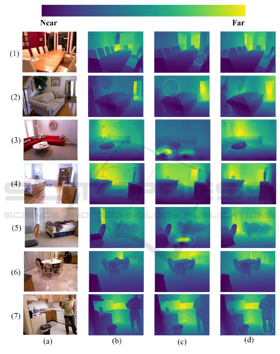
Figure 3: The ﬁgure shows: (a) each original RGB image; (b) its ground-truth depth map; (c) the depth map predicted by

DenseNet-169; (d) the depth map predicted by EfﬁcientNet.

Depth Estimation Using Weighted-Loss and Transfer Learning

785

pixels and the brighter pixels represent the far pix-

els. The results show that the EfﬁcientNet produced

more coherent results where the depth maps are more

close to the original depth maps. For example, in Fig-

ure (1,c) the circled part shows that some portion of

the chair, which was originally present in the ground

truth depth was not recovered by DenseNet, but using

the EfﬁcientNet, in Figure (1,d) this part of the image

was predicted in depth map very precisely. Similarly,

ﬁgure (2,c) shows that the plant on the background

which was present in the original image and ground

truth depth was not properly predicted, but in Figure

(2,d) the depth information about the plant is much

better. In Figure (3,c) the DenseNet predicted wrong

depth information, where the white circled portion

was predicted as far pixel, which is not the actual case

and the prediction was ﬁne in case of (3,d). Similarly,

(5,c) also has some wrong depth prediction which was

resolved in Figure (5,d). Besides this, we also ob-

served some missing information in the ground truth

depth maps. For example, in Figure (4,b) the back-

ground is a white wall, but in the ground-truth depth

map, there is an incorrect noisy pattern. Figure (4,c)

shows some missing information (depth perception of

the TV) but in Figure (4,d) both of these issues were

resolved. There is also a ground-truth error in Figure

(6,b) in which the legs of the chair are missing, but our

proposed model was able to reconstruct it from a sin-

gle RGB image with much better accuracy. Our pro-

posed model also made some wrong predictions for

example, in (7,d) the circled area is in the background,

as can be seen in (7,b) and (7,c), but our model pre-

dicted it as a near pixel.

5 CONCLUSION

Conclusion. In this study, we have proposed a sim-

ple yet promising solution for depth estimation which

is a common task in computer vision. Our primary

aim was to enhance the quantitative and visual accu-

racy of depth estimation by investigating different loss

functions and model architectures. For this purpose,

we proposed an optimized loss function, which is the

sum of three different weighted loss functions which

are MAE, Edge loss and SSIM. We reported that cho-

sen weights for the loss function, 0.6 for MAE, 0.2

for Edge Loss, and 1 for SSIM, consistently outper-

form other combinations. Additionally, we introduce

a variety of encoder-decoder based models for depth

estimation. Results showed that the EfﬁcientNet pre-

trained on ImageNet for classiﬁcation task as encoder

when used with a simple up-sampling decoder, and

our optimized loss function gave the best results. To

evaluate our proposed network, we have used both the

qualitative methods (threshold accuracy, RMSE, REL

and log

error) as well as visual or qualitative meth-

ods.

Future Work. In future work, we plan to enhance

the reliability and interpretability of depth estimation

for critical applications by adopting advanced statisti-

cal methods and explainable AI frameworks, inspired

by (Bardozzo et al., 2022) we are planning to explore

tools like Grad CAM and Grad CAM++ to provide

clear insights into our model’s decision-making pro-

cess. Furthermore, we will be using the attention

mechanism for an even better visual representation of

the depth maps and consider Pareto Front plots to fur-

ther illustrate the various weight candidates for loss

functions and how they impact the RMSE error on

the validation set.

ACKNOWLEDGEMENTS

This research is funded by Science Foundation Ire-

land under Grant number 18/CRT/6223. It is in part-

nership with VALEO.

REFERENCES

Alhashim, I. and Wonka, P. (2018). High quality monocular

depth estimation via transfer learning. arXiv preprint

arXiv:1812.11941.

Alsadik, B. and Karam, S. (2021). The simultaneous lo-

calization and mapping (slam)-an overview. Surv.

Geospat. Eng. J, 2:34–45.

Bakurov, I., Buzzelli, M., Schettini, R., Castelli, M., and

Vanneschi, L. (2022). Structural similarity index

(ssim) revisited: A data-driven approach. Expert Sys-

tems with Applications, 189:116087.

Bardozzo, F., Priscoli, M. D., Collins, T., Forgione, A.,

Hostettler, A., and Tagliaferri, R. (2022). Cross

x-ai: Explainable semantic segmentation of laparo-

scopic images in relation to depth estimation. In 2022

International Joint Conference on Neural Networks

(IJCNN), pages 1–8. IEEE.

Carvalho, M., Le Saux, B., Trouv

e-Peloux, P., Almansa, A.,

and Champagnat, F. (2018). On regression losses for

deep depth estimation. In 2018 25th IEEE Interna-

tional Conference on Image Processing (ICIP), pages

2915–2919. IEEE.

Chai, T. and Draxler, R. R. (2014). Root mean square er-

ror (rmse) or mean absolute error (mae)?–arguments

against avoiding rmse in the literature. Geoscientiﬁc

model development, 7(3):1247–1250.

VISAPP 2024 - 19th International Conference on Computer Vision Theory and Applications

786

Chen, L., Wei, H., and Ferryman, J. (2013). A survey of

human motion analysis using depth imagery. Pattern

Recognition Letters, 34(15):1995–2006.

Dong, X., Garratt, M. A., Anavatti, S. G., and Abbass, H. A.

(2022). Mobilexnet: An efﬁcient convolutional neu-

ral network for monocular depth estimation. IEEE

Transactions on Intelligent Transportation Systems,

23(11):20134–20147.

Eigen, D., Puhrsch, C., and Fergus, R. (2014). Depth map

prediction from a single image using a multi-scale

deep network. Advances in neural information pro-

cessing systems, 27.

Fu, H., Gong, M., Wang, C., Batmanghelich, K., and

Tao, D. (2018). Deep ordinal regression network

for monocular depth estimation. In Proceedings of

the IEEE conference on computer vision and pattern

recognition, pages 2002–2011.

Furukawa, R., Sagawa, R., and Kawasaki, H. (2017). Depth

estimation using structured light ﬂow–analysis of pro-

jected pattern ﬂow on an object’s surface. In Proceed-

ings of the IEEE International conference on com-

puter vision, pages 4640–4648.

Garg, R., Bg, V. K., Carneiro, G., and Reid, I. (2016). Unsu-

pervised cnn for single view depth estimation: Geom-

etry to the rescue. In Computer Vision–ECCV 2016:

14th European Conference, Amsterdam, The Nether-

lands, October 11-14, 2016, Proceedings, Part VIII

14, pages 740–756. Springer.

Godard, C., Mac Aodha, O., and Brostow, G. J. (2017).

Unsupervised monocular depth estimation with left-

right consistency. In Proceedings of the IEEE con-

ference on computer vision and pattern recognition,

pages 270–279.

Hao, Z., Li, Y., You, S., and Lu, F. (2018). Detail preserving

depth estimation from a single image using attention

guided networks. In 2018 International Conference

on 3D Vision (3DV), pages 304–313. IEEE.

Hirschmuller, H. and Scharstein, D. (2008). Evaluation of

stereo matching costs on images with radiometric dif-

ferences. IEEE transactions on pattern analysis and

machine intelligence, 31(9):1582–1599.

Laina, I., Rupprecht, C., Belagiannis, V., Tombari, F., and

Navab, N. (2016). Deeper depth prediction with fully

convolutional residual networks. In 2016 Fourth inter-

national conference on 3D vision (3DV), pages 239–

248. IEEE.

Li, B., Dai, Y., and He, M. (2018). Monocular depth es-

timation with hierarchical fusion of dilated cnns and

soft-weighted-sum inference. Pattern Recognition,

83:328–339.

Masoumian, A., Rashwan, H. A., Cristiano, J., Asif, M. S.,

and Puig, D. (2022). Monocular depth estimation us-

ing deep learning: A review. Sensors, 22(14):5353.

Mauri, A., Khemmar, R., Decoux, B., Benmoumen, T.,

Haddad, M., and Boutteau, R. (2021). A compara-

tive study of deep learning-based depth estimation ap-

proaches: Application to smart mobility. In 2021 8th

International Conference on Smart Computing and

Communications (ICSCC), pages 80–84. IEEE.

Murez, Z., Van As, T., Bartolozzi, J., Sinha, A., Badri-

narayanan, V., and Rabinovich, A. (2020). Atlas: End-

to-end 3d scene reconstruction from posed images. In

Computer Vision–ECCV 2020: 16th European Con-

ference, Glasgow, UK, August 23–28, 2020, Proceed-

ings, Part VII 16, pages 414–431. Springer.

Patil, V., Sakaridis, C., Liniger, A., and Van Gool, L. (2022).

P3depth: Monocular depth estimation with a piece-

wise planarity prior. In Proceedings of the IEEE/CVF

Conference on Computer Vision and Pattern Recogni-

tion, pages 1610–1621.

Paul, S., Jhamb, B., Mishra, D., and Kumar, M. S. (2022).

Edge loss functions for deep-learning depth-map. Ma-

chine Learning with Applications, 7:100218.

Sikder, A. K., Petracca, G., Aksu, H., Jaeger, T., and Ulu-

agac, A. S. (2021). A survey on sensor-based threats

and attacks to smart devices and applications. IEEE

Communications Surveys & Tutorials, 23(2):1125–

1159.

Silberman, N., Hoiem, D., Kohli, P., and Fergus, R. (2012).

Indoor segmentation and support inference from rgbd

images. In Computer Vision–ECCV 2012: 12th Euro-

pean Conference on Computer Vision, Florence, Italy,

October 7-13, 2012, Proceedings, Part V 12, pages

746–760. Springer.

Tang, S., Tan, F., Cheng, K., Li, Z., Zhu, S., and Tan, P.

(2019). A neural network for detailed human depth

estimation from a single image. In Proceedings of the

IEEE/CVF International Conference on Computer Vi-

sion, pages 7750–7759.

Torralba, A. and Oliva, A. (2002). Depth estimation from

image structure. IEEE Transactions on pattern analy-

sis and machine intelligence, 24(9):1226–1238.

Wang, Z., Bovik, A. C., Sheikh, H. R., and Simoncelli, E. P.

(2004). Image quality assessment: from error visi-

bility to structural similarity. IEEE transactions on

image processing, 13(4):600–612.

Yan, S., Yang, J., Leonardis, A., and K

ainen, J. (2021).

Depth-only object tracking. In British Machine Vision

Conference.

Yang, Y., Wang, Y., Zhu, C., Zhu, M., Sun, H., and Yan, T.

(2021). Mixed-scale unet based on dense atrous pyra-

mid for monocular depth estimation. IEEE Access,

9:114070–114084.

Yue, H., Zhang, J., Wu, X., Wang, J., and Chen, W. (2020).

Edge enhancement in monocular depth prediction. In

2020 15th IEEE Conference on Industrial Electronics

and Applications (ICIEA), pages 1594–1599. IEEE.

Zhao, C., Sun, Q., Zhang, C., Tang, Y., and Qian, F. (2020).

Monocular depth estimation based on deep learning:

An overview. Science China Technological Sciences,

63(9):1612–1627.

Depth Estimation Using Weighted-Loss and Transfer Learning

787