Particle-Wise Higher-Order SPH Field Approximation for DVR
Jonathan Fischer
1
, Martin Schulze
1
, Paul Rosenthal
2 a
and Lars Linsen
3 b
1
Department of Computer Science, Chemnitz Technical University, Str. der Nationen 62, 09111 Chemnitz, Germany
2
Institute for Visual and Analytic Computing, University of Rostock, Albert-Einstein-Str. 22, 18059 Rostock, Germany
3
Institute of Computer Science, University of M
¨
unster, Einsteinstr. 62, 48149 M
¨
unster, Germany
Keywords:
Scientific Visualization, Ray Casting, Higher-Order Approximation, Volume Rendering, Scattered Data, SPH.
Abstract:
When employing Direct Volume Rendering (DVR) for visualizing volumetric scalar fields, classification is
generally performed on a piecewise constant or piecewise linear approximation of the field on a viewing ray.
Smoothed Particle Hydrodynamics (SPH) data sets define volumetric scalar fields as the sum of individual par-
ticle contributions, at highly varying spatial resolution. We present an approach for approximating SPH scalar
fields along viewing rays with piecewise polynomial functions of higher order. This is done by approximating
each particle contribution individually and then efficiently summing the results, thus generating a higher-order
representation of the field with a resolution adapting to the data resolution in the volume.
1 INTRODUCTION
Introduced by Gingold and Monaghan (Gingold and
Monaghan, 1977) and independently by Lucy (Lucy,
1977), Smoothed Particle Hydrodynamics (SPH) is
a group of methods for simulating dynamic mechan-
ical processes, typically fluid or gas flows but also
solid mechanics. The objective matter is modeled
by means of particles, each representing a small por-
tion of a simulated substance and attributed a specific
mass, density, and other physical measures.
These discrete and scattered particles define scalar
and vector fields on the spatial continuum through
an interpolation rule, determining a physical field as
the sum of the isotropic contributions of the particles,
each following a smooth function only of the distance
from the particle position, called the kernel function.
As an example, we refer to the SPH kernel function
defined by the cubic B-spline (Rosswog, 2009)
w
(r) =
1
4π





(2 − r)
3
− 4(1 − r)
3
, 0 ≤ r < 1
(2 − r)
3
, 1 ≤ r < 2
0, 2 ≤ r .
(1)
In this work, we assume the kernel function to have
compact support. We consider this to be a mi-
nor restriction because kernel functions with compact
support are appreciated in the SPH community for
a
https://orcid.org/0000-0001-9409-8931
b
https://orcid.org/0000-0002-6168-8748
bounding the particles’ volumes of influence. Obvi-
ously, by simply defining some cut-off value as upper
bound, any kernel function can be supported. Given
such a function, a particle’s contribution to a scalar
field can be expressed as
µα
ρζ
3
w

∥
x − χ
∥
ζ

for the particle’s position χ, mass µ, target field value
α, density ρ, and smoothing radius ζ. While µ, α,
and ρ serve as simple multiplicative constants, defin-
ing only the amplitude of the contribution, ζ radially
scales the domain and thus defines the radius of the
particle’s volume of influence.
Direct Volume Rendering (DVR): has a long-
standing tradition for visualizing scalar volumetric
fields (Drebin et al., 1988) and is commonly imple-
mented as a ray casting method. It builds on assign-
ing visual characteristics, representing features of the
field, to the target domain volume and then rendering
it by casting viewing rays through the volume. The
color of each pixel of the output image is the result of
simulating the behavior of light traveling through the
volume along a ray in opposite viewing direction.
Said visual characteristics, usually comprising
light emission and absorption, are computed from lo-
cal target field characteristics, like values or gradients,
in a process called classification (Max, 1995). It is
commonly employed based on a piecewise constant
or piecewise linear approximation of the target scalar
Fischer, J., Schulze, M., Rosenthal, P. and Linsen, L.
Particle-Wise Higher-Order SPH Field Approximation for DVR.
DOI: 10.5220/0012460500003660
Paper published under CC license (CC BY-NC-ND 4.0)
In Proceedings of the 19th International Joint Conference on Computer Vision, Imaging and Computer Graphics Theory and Applications (VISIGRAPP 2024) - Volume 1: GRAPP, HUCAPP
and IVAPP, pages 717-725
ISBN: 978-989-758-679-8; ISSN: 2184-4321
Proceedings Copyright © 2024 by SCITEPRESS – Science and Technology Publications, Lda.
717

field along the ray.
Direct volume rendering of astronomical SPH
data was first performed by incorporating contribu-
tions of both grid and particle data into the optical
model (K
¨
ahler et al., 2007). Efficient full-featured
DVR applied directly to large SPH data sets on com-
modity PC hardware has first been managed by re-
sampling the scalar fields to a perspective grid held
in a 3-d texture for each rendering frame (Fraedrich
et al., 2010). Later, DVR for large scattered data was
proposed to be performed on the CPU by Knoll et al.
(Knoll et al., 2014) and mostly applied to molecular
dynamics. Although employing radial basis function
kernel (RBF) interpolation similar to the SPH case,
they focus on the very special task of rendering a sur-
face defined by a density field. This is in line with
more recent contributions in rendering SPH data, such
as (Hochstetter et al., 2016) or (Oliveira and Paiva,
2022), targeting only simulated fluids.
The approaches for volume-rendering arbitrary
SPH fields employ equidistant sampling of the target
field along viewing rays and acting on a piecewise lin-
ear approximation of it, which, depending on the local
particle density, may miss detailed features in regions
of high particle density, or oversample particles with
large smoothing length in sparse regions.
Thus, in this work, we explore the capabilities and
limitations of approximating SPH scalar fields with
higher-order piecewise polynomial functions, whose
resolution adapts to the local resolution of the given
particle data. The higher-order approximations may
facilitate quantitatively more accurate output images
at a worthwhile cost.
2 METHOD OVERVIEW
As SPH interpolation defines the target scalar field
as the sum of particle contributions to it, our con-
cept builds on approximating each individual parti-
cle contribution on a viewing ray and then employing
the sum of these approximations. Although summing
an indefinite number of piecewise polynomial func-
tions may seem like a task of quadratic complexity not
amenable to GPU processing, we encode these func-
tions in a way reducing the summation to a simple
sorting task. Our method comprises three passes:
1. For each particle, approximate its contribution to
all relevant viewing rays.
2. For each ray, sort the contribution data assigned to
it with respect to the distance from the viewer.
3. For each ray, accumulate the contributions along
the ray, classify and composite the result.
In the remainder of this section, we declare our
concept of representing piecewise polynomial func-
tions and show how these can be processed during the
compositing sweep. In Section 3, we present a way to
efficiently compute optimal approximations for single
particle contributions during the first sweep. In Sec-
tion 4, we then describe a pitfall that our higher-order
approximation scheme involves and develop an im-
provement of our method to overcome this difficulty.
Finally, in Section 5, we analyze the approximation
errors implied by our scheme and discuss the choice
of the major parameters like the approximation order,
before concluding our work in Section 6.
Localized Difference Coefficients. A real polyno-
mial function A : R → R of order D is generally rep-
resented by its coefficients, i. e., numbers a
d
∈ R such
that
A
(t) =
∑
D
d=0
a
d
t
d
. They provide a direct image of
how the function and all its derivatives behave at t = 0
since the d
th
derivative of A at t = 0 amounts to d!a
d
.
If we wanted to know the value or derivative of order
d at some other t
∗
, we could compute it as
A
(d)
(t
∗
) =
D
∑
j=d
j!
( j − d)!
a
j
t
j−d
∗
= d!
D
∑
j=d

j
d

a
j
t
j−d
∗
,
which shows that the real numbers
a
∗d
=
D
∑
j=d

j
d

a
j
t
j−d
∗
represent the order-d behavior of A at t = t
∗
just as the
a
d
do at t = 0. In fact, A can be expressed using these
localized coefficients as
A
(t) =
D
∑
d=0
a
∗d
(t −t
∗
)
d
.
Now, a continuous piecewise polynomial function
is defined by a sequence of border arguments t
0
< t
1
<
... and several polynomial functions A
0
,A
1
,... such
that each polynomial function A
k
is applied in its re-
spective interval [t
k
,t
k+1
].
If we were representing each polynomial A
k
by its
coefficients, summing several piecewise polynomial
functions would require tracking the applicable poly-
nomials for each resulting argument interval and sum-
ming their coefficients.
Instead, we save for each border argument t
k
the
change that the overall function performs in all orders.
Specifically, we save the localized coefficients of the
difference between the polynomials A
k
applicable on
the right of t
k
and A
k−1
applicable on its left.
Thus, when saving a piecewise polynomial ap-
proximation of order D along a viewing ray, we en-
code it as a sequence of knots
(t
k
, ˆa
k0
,..., ˆa
kD
), k = 0, 1, . ..
IVAPP 2024 - 15th International Conference on Information Visualization Theory and Applications
718

consisting of a ray parameter t
k
defining the knot po-
sition on the ray and localized difference coefficients
ˆa
k0
,..., ˆa
kD
, such that
A
k
(t) − A
k−1
(t) =
D
∑
d=0
ˆa
kd
(t −t
k
)
d
.
Summing several piecewise polynomials encoded this
way amounts to nothing more than sorting their joint
knots for increasing knot positions. The resulting ap-
proximation can then be processed piece by piece, re-
trieving the localized coefficients a
k0
,...,a
kD
of each
piece polynomial A
k
at its left boundary argument t
k
from the ones of the last piece according to the updat-
ing rule
a
kd
= ˆa
kd
+
D
∑
j=d

j
d

a
(k−1) j
(t
k
−t
k−1
)
j−d
(2)
for d = 0,. . . , D, which is a computation of constant
complexity per piece, irrespective of the number of
particles contributing.
3 APPROXIMATING SINGLE
PARTICLE CONTRIBUTIONS
3.1 Deduction from Unit Particle
Since the same SPH kernel function is applied for all
particles, their contributions to the volume differ in
only a few scaling and translation parameters, namely
their position χ, mass µ, density ρ, smoothing radius
ζ, and applicable scalar field attribute α.
χ
b
v
1
x

t
χ

Λζ
qζ
x(t) = b + tv


t − t
χ


Figure 1: Sketch of measures involved in the positional re-
lationship between viewing ray and particle. The volume of
influence of a particle with smoothing length ζ is intersected
by a viewing ray, defined by base point b and unit direction
vector v. The particle’s contribution on the ray at a point
x(t) is determined by its distance to the particle position χ.
We denote by q the upper bound of the kernel function’s
support, such that qζ is the radius of the particle’s volume
of influence.
To model a viewing ray, we fix a straight line
with vector equation x(t) = b +tv for some base point
b ∈ R
3
, unit direction vector v ∈ R
3
, and parameter
t ∈ R. We consider a normalized particle, i. e., one
of unit mass, unit density, unit field attribute, and unit
smoothing radius. Assuming the base point b on the
ray is the one closest to the particle position, the nor-
malized particle’s contribution to this line is
B
Λ
(t) =
w

p
Λ
2
+t
2

,
where Λ is the distance between the particle’s position
and the line. Then, the contribution of a specific data
particle on a ray at distance Λζ from its position χ
amounts to
µα
ρζ
3
B
Λ

t − t
χ
ζ

,
where t
χ
is the parameter of the point on the ray clos-
est to the particle position and Λ =
1
ζ


χ − x

t
χ



. The
situation is depicted in Figure 1.
Finding optimal piecewise polynomial approxi-
mations for B
Λ
for all Λ within the SPH kernel’s
support suffices to generate optimal approximations
for any particle by just translating and scaling it in
the same way. For quick access, we thus prepare a
look-up table containing the localized difference co-
efficients of order-D approximations of B
Λ
for many
equidistant values of Λ. In the remainder of this sec-
tion, we show how we can find these optimal approx-
imations.
3.2 Optimization Problem Definition
Before we can find optimal approximations, we need
to define what optimality shall mean in this context.
Specifically, we have to settle on:
1. The space of eligible candidates, i. e., the condi-
tion of what we want to consider a feasible ap-
proximation.
2. The error measure defining whether one approxi-
mation is better than another.
The main restriction on the space of eligible approx-
imation candidates is the imposition of a maximum
polynomial degree D, i.e, the order of approximation,
and the number K of non-trivial polynomial pieces
per particle, i. e., the number of non-zero polynomials
defining the approximation of a single particle. We
dedicate Section 5 to evaluating choices of D and K
but leave them unspecified for now. Beyond that, we
demand that our approximations shall be continuous
and even functions with compact support. This seems
reasonable, as our approximation target B
Λ
also has
these properties.
For measuring the approximating quality of any
piecewise polynomial function candidate S : R → R,
Particle-Wise Higher-Order SPH Field Approximation for DVR
719

we apply its L
2
distance to B
Λ
, i. e., we seek to mini-
mize the approximation error
E
Λ
(S) =
∥
S − B
Λ
∥
2
=


Z
R
[
S
(t) − B
Λ
(t)]
2
dt


1
2
. (3)
In contrast to the supremum norm often used in ap-
proximation theory, this error measure punishes not
only the maximum pointwise deviation from the tar-
get, but also the length of segments of high deviation.
Moreover, another advantage of the L
2
norm is its as-
sociated inner product, which allows us to generate
a closed-form solution of the optimal approximation
and its error value as a function only of the knot po-
sitions, as shown in Section 3.3. We then find opti-
mal knot positions through standard non-linear opti-
mization as explained in Section 3.4. Detailed proofs
of our findings can be found in the appendix of our
preprint (Fischer et al., 2024) hosted on arxiv.org.
3.3 Solution for Fixed Knot Positions
As a prerequisite for finding truly optimal approxima-
tions, we first handle the case of arbitrary fixed knot
positions. Due to our evenness requirement, the neg-
ative knot positions are determined from the positive
ones. Hence, our optimization domain is the set of
even continuous piecewise polynomial functions with
compact support, maximal degree D, maximal num-
ber of non-trivial pieces K, and positive knot positions
θ
1
,...,θ
⌈
K
/2
⌉
. We denote this set by S .
Consider the vector space L
2
(R) of square-
integrable functions R → R, which by the Riesz-
Fischer theorem is complete with respect to the L
2
norm and therefore a Hilbert space when equipped
with the inner product
⟨
A,B
⟩
=
Z
R
A
(t)
B
(t)dt for A,B ∈ L
2
(R),
which induces the L
2
norm
∥
A
∥
2
=
p
⟨
A,A
⟩
. The ap-
proximation target B
Λ
is clearly an element of L
2
(R)
as it is continuous and has compact support.
For any A,B ∈ L
2
(R), B ̸≡ 0, we denote by
proj
B
(A) =
⟨
A,B
⟩
⟨
B,B
⟩
B
the orthogonal projection of A on B.
As we will see shortly, S is a subspace of L
2
(R)
of finite dimension

KD
2

, for which we can compute
an orthogonal basis A, which in turn we can use to
calculate the orthogonal projection of B
Λ
on S as
S
Λ
=
∑
A∈A
proj
A
(B
Λ
). (4)
It is easy to show that S
Λ
is the unique error-
optimal approximation of B
Λ
among the elements of
S (proof in (Fischer et al., 2024)). Therefore, all
we need for computing the optimal approximation for
fixed knot positions is a suitable orthogonal basis.
We specify a non-orthogonal basis as a starting
point here: Let J be the set of pairs (k,d) of posi-
tive integers k ≤
⌈
K
/2
⌉
and d ≤ D but excluding ele-
ments (1,d) for uneven d if K is uneven. Then the set
˜
A =

˜
A
kd
: (k, d) ∈ J

of functions
˜
A
kd
(t) =







1 if
|
t
|
≤ θ
k−1
1 −

|
t
|
−θ
k−1
θ
k
−θ
k−1

d
if θ
k−1
≤
|
t
|
≤ θ
k
0 if
|
t
|
≥ θ
k
is a basis of S (proof in (Fischer et al., 2024)).
Given
˜
A, we convert it into an orthogonal ba-
sis A =
{
A
kd
: (k, d) ∈ J
}
by employing the Gram-
Schmidt process. Specifically, we recursively set
A
k
∗
d
∗
=
˜
A
d
∗
k
∗
−
∑
(k,d)∈J
k<k
∗
∨(k=k∧d<d
∗
)
proj
A
kd

˜
A
d
∗
k
∗

in lexicographical order of pairs (k
∗
,d
∗
) ∈ J .
3.4 Optimal Knot Positions
While we can directly compute optimal approxima-
tions for given knot positions as shown above, finding
error-optimal knot positions is a nonlinear optimiza-
tion problem over the variables θ
1
,...,θ
⌈
K
/2
⌉
.
The objective function E
Λ
is continuous within the
interior of the feasible domain defined by the con-
straints 0 < θ
1
< ··· < θ
⌈
K
/2
⌉
, due to the continuity
of the inner product and of the constructed basis with
respect to the θ
k
, which would even hold for a dis-
continuous SPH kernel function. Also, we can expect
to find a global optimizer within the interior of the
feasible domain, i. e., without any of the constraints
being active, because an equality of any two variables
would be equivalent to a reduction of the number of
non-zero pieces, diminishing the freedom for approx-
imating and therefore resulting in higher or equal er-
ror. Hence, if a local optimum was attained at the fea-
sible domain border, it could not be isolated because
shifting one of the colliding θ
k
and defining the poly-
nomials on both of its sides to be equal would result
in the same approximation function and therefore in
the same error value.
While evaluating E
Λ
could be done following the
steps above for every set of fixed θ
1
,...,θ
⌈
K
/2
⌉
, it is
worthwhile to only fix K and D and perform the pro-
cess in a symbolic manner, generating an explicit for-
mula of the objective error function, which can later
IVAPP 2024 - 15th International Conference on Information Visualization Theory and Applications
720

be evaluated for any knot positions and distance pa-
rameter Λ. The generation of a closed-form represen-
tation of an orthogonal basis for variable knot posi-
tions and Λ has to be done only once as it does not
depend on the SPH kernel used. However, the ex-
plicit expression of the approximation error follow-
ing (4) requires closed-form solutions of the integrals
defining the inner products
⟨
A,B
Λ
⟩
for orthogonal ba-
sis functions A. In the case of an SPH kernel defined
by a continuous piecewise polynomial function such
as the cubic B-spline kernel (1), this can clearly be
achieved. In any case, as the symbolic computations
are rather involved, computer algebra systems are of
great help during this preparatory process.
We have conducted this process for the cubic B-
spline kernel, going to considerable length to find a
global optimizer for many discrete Λ. For Λ close to
the upper bound q, however, we have found the evalu-
ation of some of the formulae to become instable. To
obtain reliable results, we employed the GNU MPFR
library to perform the computations in multiple preci-
sion arithmetic. Since we have not encountered any
severe problems during these optimizations, we have
reason to hope they are manageable for any piecewise
polynomial SPH kernel function.
4 QUANTIZATION TO PREVENT
HIGHER-ORDER ERRORS
4.1 Higher-Order Rounding Error
Propagation
For the stated efficiency reasons, the recursive com-
putation of polynomial coefficients according to (2)
is an integral component to our particle-wise approx-
imation approach. However, it comes at a substan-
tial price which may not be obvious at first glance.
Directly applying (2) during the compositing sweep
using floating-point numbers is problematic because
rounding errors are propagated at higher order from
front to back along the viewing ray, resulting in unre-
liable coefficients especially for higher t.
To illustrate the issue, consider a piecewise poly-
nomial function modeling the contribution of a small
number of particles. Clearly, the last piece polyno-
mial of this approximation should be the zero polyno-
mial. However at its starting knot, its value is most
probably not computed to be zero but some value
close to zero, due to rounding errors in the compu-
tation. Although this zeroth-order distortion may be
negligible by itself, small rounding errors in higher-
order terms cause large errors further down the ray.
We may thus find the polynomial’s value to have
grown far from zero for larger t.
The direct effect of these errors is an unstable re-
sult: When using a transfer function with focus on
lower attribute values typically reached just before
leaving the volumes of influence of the last contribut-
ing particles, the resulting pixel colors are highly un-
stable and the generated images show strong “sprin-
kling” artifacts, as shown in Figure 2 (a). Hence,
solving this problem is indispensable if we want our
higher-order ray casting concept to be of any use.
There are several conceivable measures for allevi-
ation. One is to limit the maximum distance on the
ray that the error may use to grow by introducing a
number of special reinitialization knots at predeter-
mined t on all rays, as performed for the rendering
of Figure 2 (b). When processing a particle during
the first sweep, in addition to the knots encoding its
higher-order approximation as difference coefficients,
we also add to all covered reinitialization knots the
localized coefficients of this particle’s contributions.
Later when processing the sorted sequence of knots,
whenever we encounter a reinitialization knot, we di-
rectly take the coefficients attached to it instead of
computing the coefficients following the update rule
(2), thus eliminating the effect of past errors for fu-
ture pieces. However, this approach not only intro-
duces the complexity of two different kinds of knots
but also can only partially solve the problem. Besides,
defining how many reinitialization knots to utilize is
non-trivial.
Clearly, an alternative would be to avoid the cause
of higher-order error propagation altogether and pro-
ceed to a direct, possibly localized, coefficient repre-
sentation of the polynomials, considering for the com-
putation of each result piece only the contributions
with overlapping support. While this would most
probably facilitate stable results, it would mean ac-
cepting the expense of determining for each piece the
set of relevant contributions.
4.2 Exact Arithmetic Through
Quantization
We propose yet another approach to fully avoid
rounding errors during the computation of (2), namely
by transferring all involved quantities from floating-
point to fixed-point numbers, which allow an exact
arithmetic. More precisely, we slightly shift all num-
bers encoding the individual contribution approxima-
tions into integer multiples of some quantum values,
a process we call quantization. While this increases
the approximation errors for the individual contribu-
tions, the update operations in (2) are reduced to exact
Particle-Wise Higher-Order SPH Field Approximation for DVR
721

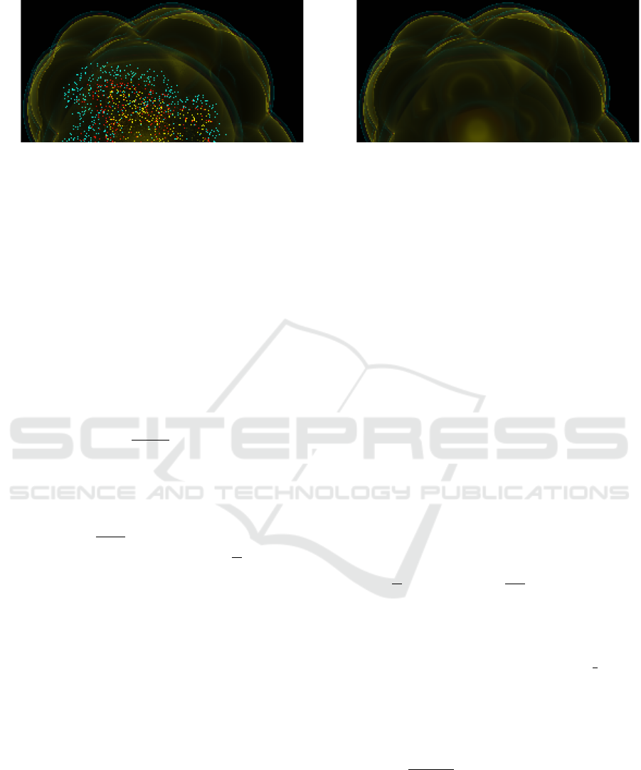
(a) (b)
Figure 2: Extracts of sample renderings of the temperature field of an SPH data set using our higher-order SPH field ap-
proximation scheme and a transfer function emphasizing three rather low temperature value regions by mapping them to an
emission of blue, yellow, and red light. All computations are performed in single precision on the GPU.
(a) clearly shows “sprinkling” artifacts caused by higher-order rounding error propagation, which “randomly” cause the field
approximation on the ray to stay within one of the highlighted temperature regions far “behind” the particle cluster.
(b) shows the result of employing 10 slices of reinitialization to mitigate the problem.
integer manipulations.
Adhering to the notation used in (2), the val-
ues to be quantized are the elements of the knots
(t
k
, ˆa
k0
,..., ˆa
kD
) and the localized coefficients a
kd
.
We thus seek to fix real quantum values τ > 0 and
ς
d
> 0 for d = 0,...,D such that t
k
≈
¯
t
k
τ for some
¯
t
k
∈ N and ˆa
kd
≈
¯
ˆa
kd
ς
d
, a
kd
≈ ¯a
kd
ς
d
for integers
¯
ˆa
kd
and ¯a
kd
. The quantized knots can then be encoded as
the integer components

¯
t
k
,
¯
ˆa
k0
,...,
¯
ˆa
kD

.
Written in these terms, (2) becomes
¯a
kd
=
¯
ˆa
kd
+
D
∑
j=d

j
d

ς
j
τ
j−d
ς
d
¯a
(k−1) j
(
¯
t
k
−
¯
t
k−1
)
j−d
,
which we have to guarantee to result in an integer
for arbitrary integer values of previously computed
(
¯
t
k
−
¯
t
k−1
) and ¯a
(k−1) j
. This can only be accomplished
by requiring

j
d

ς
j
τ
j−d
ς
d
∈ Z for all d and j ≥ d, which
we can fulfill by simply setting ς
d
=
ς
τ
d
for all d,
where we abbreviate ς = ς
0
. This leaves us with only
two quantum values: one length quantum τ and one
field value quantum ς. We show our strategy of choos-
ing the two in Section 4.4.
However, we first specify in Section 4.3 how we
set up the quantized knot positions
¯
t
k
and difference
coefficients
¯
ˆa
kd
, which later form the input of the co-
efficients update rule (2), now reduced to the integer-
only representation
¯a
kd
=
¯
ˆa
kd
+
D
∑
j=d

j
d

¯a
(k−1) j
(
¯
t
k
−
¯
t
k−1
)
j−d
. (5)
In Section 4.3, we specify how we compute quantized
knots from the particle data and the optimal unit parti-
cle approximations in the look-up table while in Sec-
tion 4.4 we explain how we find appropriate quantum
values ς and τ. Detailed proofs and derivations can be
found in the appendix to our preprint (Fischer et al.,
2024) hosted on arxiv.org.
4.3 Setting Quantized Knots
In order to not introduce higher-order errors through
the back door after all, we have to ensure that the input
to the integer computations does not contain such er-
rors already. Each individual particle approximation
has to have compact support, i. e., its knots have to
exactly neutralize each other. This guides us to com-
pute the knots of single particle contributions accord-
ing to the following rules (derivation in (Fischer et al.,
2024)).
Given a particle with attributes µ, ρ, ζ , and α, po-
sitioned at distance Λζ from the ray with closest point
parameter t
χ
, we select from the look-up table the op-
timal normalized positive knot positions θ
k
and local-
ized difference coefficients ˆs
kd
corresponding to the
normalized distance closest to Λ, all in floating-point
representation.
We then set the knot position quantum counts to
¯
t
0
=

t
χ
τ

and
¯
t
k
=
¯
t
0
+

ζθ
k
τ

,
¯
t
−k
= 2
¯
t
0
−
¯
t
k
for k = 1,...,
⌈
K
/2
⌉
, where we use
⌈
·
⌋
, a notation in-
spired by (Hastad et al., 1989, page 860), to refer to
just a usual nearest integer rounding function. In this
context it is irrelevant whether we round z +
1
2
to z or
to z + 1 for z ∈ Z.
Then, for k ≥ 1, except for k = 1 and uneven d if
K is uneven, the quantized localized difference coef-
ficients are computed as
¯
ˆa
kd
=

τ
d
µα ˆs
kd
ςρζ
d+3

and
¯
ˆa
−kd
= (−1)
d+1
¯
ˆa
kd
.
In case of K being even, there is a middle knot
with possibly non-zero coefficients
¯
ˆa
0d
= −2
−1
∑
k=−
⌈
K
/2
⌉
D
∑
j=d

j
d

¯
ˆa
k j
(
¯
t
0
−
¯
t
k
)
j−d
IVAPP 2024 - 15th International Conference on Information Visualization Theory and Applications
722

for uneven d. Otherwise, there is no middle knot, i. e.,
¯
ˆa
0d
= 0 for all d, but we set
¯
ˆa
−1d
= −
−2
∑
k=−
⌈
K
/2
⌉
¯
ˆa
kd
−
D
∑
j=d+1

j
d

−1
∑
k=−
⌈
K
/2
⌉
¯
ˆa
k j
(
¯
t
0
−
¯
t
k
)
j−d
and
¯
ˆa
1d
= (−1)
d+1
¯
ˆa
−1d
in descending order of un-
even d.
4.4 Specifying Quantum Values
Computing optimal quantum values requires the defi-
nition of a manageable error measure for minimiza-
tion. In our attempts to measure the changes to
the field approximation originating from quantiza-
tion, we have developed the data-independent and
ray-independent relative quantization error estimate
(derivation in (Fischer et al., 2024))
Q
D
(τ,ς) =
1
4κ
s
κ
′2
τ
2
+
D
∑
d=0
2q
2d+3
(2d + 1) (2d + 3)
·
ς
2
τ
2d
,
where q is the upper bound of the kernel function’s
support and we have abbreviated the constants
κ =


4π
∞
Z
t=0
[t
w
(t)]
2
dt


1
2
and
κ
′
=


q
Z
0
Λ
Z
R

d
dt
B
Λ
(t)

2
dt dΛ


1
2
,
which only depend on the SPH kernel.
Q
D
clearly grows with ς, which is reasonable be-
cause the smaller we set ς, the closer the quantized
approximations cat get to the optimal ones. However,
smaller ς require larger integer values ¯a
kd
and
¯
ˆa
kd
.
Hence, to guard against integer overflow, we propose
to set it to the optimal lower bound
ς =
a
max
INT MAX
,
where INT MAX is the maximum representable in-
teger for an integer bit-length yet to be chosen, and
a
max
an overall upper bound of the values expected to
occur in the approximation, which can be generated
by a short analysis of the data set to be visualized.
The situation is not as straight-forward for the
length quantum τ. On the one hand, large τ result in
large quantization errors by distorted knot positions.
On the other hand, small τ mean large higher-order
quantum values ς
d
, as we have seen in Section 4.2.
However, given ς, it is easy to show that Q
D
(τ,ς) is
a convex function with respect to τ, whose minimizer
can be found by common root-finding methods (proof
in (Fischer et al., 2024)).
We have to note, though, while Q
D
(τ,ς) estimates
the relative quantization error of a normalized parti-
cle, the quantization error for a particle from the data
set is better represented by
Q
D

1
ζ
τ,
ρζ
3
µα
ς

,
i. e., it depends on the particle attributes. Thus, for the
purpose of determining a suitable global τ, we first
specify “representative” attributes µ
repr
, ρ
repr
, ζ
repr
,
and α
repr
of the data set to be visualized. These could
be, for example, average or mean values or the at-
tributes chosen from any particle in a region of inter-
est. Afterwards, abbreviating φ
repr
=
µ
repr
α
repr
ρ
repr
ζ
3
repr
, we set
τ to minimize Q
D

τ
ζ
repr
,
ς
φ
repr

.
5 CHOOSING APPROXIMATION
DIMENSIONS
Having set forth our quantized higher-order approx-
imation field concept, the question remains how to
choose its most fundamental parameters: the approxi-
mation order D, the number of non-trivial polynomial
pieces per particle K, and the bit length defining the
maximum representable integer INT MAX. All three
parameters can significantly impact both approxima-
tion accuracy and performance. While the quality
of any configuration (D,K,INT
MAX) ultimately re-
quires thorough testing to be readily evaluated, we do
want to provide an overview in theory here.
5.1 Performance Implications
The method’s asymptotic complexity with respect to
K and D is easily seen: K has linear impact on the
number of knots per ray and therefore a linearith-
mic one on the overall process time due to the search
sweep. The overall time effect of D is quadratic since
both the number of coefficients to be updated and the
number of operations for each coefficient update ac-
cording to (5) grow linearly with D.
The performance implications of the integer bit
length require special attention. In spite of the focus
on floating-point performance, modern GPUs intrin-
sically support calculations on integer types of 16-bit
and 32-bit lengths. For 32-bit integers, the through-
put of additions is comparable to 32-bit floating-point
operations while multiplications are commonly pro-
cessed about five times slower. 64-bit integer opera-
tions are formally supported in some GPU program-
Particle-Wise Higher-Order SPH Field Approximation for DVR
723

ming contexts (Vulkan API, OpenCL, CUDA, exten-
sion of GLSL) but seem to be always emulated in soft-
ware based on 32-bit operations.
Such an emulation can easily be constructed for
integer types of any size, which means that in the-
ory we can go with arbitrarily small quantum values,
albeit at a high price performance-wise. To get an im-
pression about the performance implications of using
such long integers, we have analysed such algorithms.
Compared to 32-bit integers, our results show a cost
increase by a factor of roughly 9 for bit-length 64,
24 for 96 bit, and 45 for 128 bit, although we expect
64-bit integers to be especially well-optimized in the
implementations by GPU vendors.
To be able to decide whether these cost factors are
worthwhile and, consequently, choose adequate quan-
tum values, we have to form an idea of the quality im-
plications of smaller or larger integer sizes. In other
words, we have to relate the quantization cost to the
quantization error.
5.2 Combined Accuracy Measure
In order to estimate the overall accuracy implications
of D, K, and INT MAX, we combine the error esti-
mate for piecewise polynomial approximation and the
one for quantization.
In Section 3.2, we have already defined the error
E
Λ
(S) for a non-quantized approximation along a ray
with normalized distance Λ. To become independent
from Λ and the screen resolution, we integrate the op-
timal per-ray error over all viewing rays in one direc-
tion. We then divide it by the L
2
norm κ of a normal-
ized particle’s contribution to arrive at the per-particle
relative error for higher-order approximation
E
K,D
=
1
κ


2π
q
Z
0
ΛE
2
Λ
(S
Λ
)dΛ


1
2
,
where we have used S
Λ
to refer to the optimal ap-
proximation at distance Λ with optimal knot posi-
tions. As we are given these approximations only im-
plicitly through a minimization process, we compute
E
K,D
only approximately as a Riemann sum. It con-
stitutes a precise relative approximation error measure
for any particle, not just for the normalized ones.
By contrast, the quantization error is difficult to
quantify exactly, due to the statistical and rather com-
plex distortion caused by quantization. We thus
content ourselves with the rather rough estimate
Q
D

τ
ζ
repr
,
ς
φ
repr

defined in Section 4.4. While this
measure is already in the form of a per-particle rel-
ative error derived from an all-rays integration similar
to the one for E
K,D
above, it has the disadvantage of
apparently depending on τ, ς, and the particle data.
Fortunately, a closer look reveals that the only prop-
erty of the data set that Q
D
really depends on is
a
max
φ
repr
,
i. e., the ratio between a “representative” particle’s
factor to the SPH kernel and an upper bound of the
target field value. It is a measure for the variance of
the target scalar field. Fixing this value at, say, 10
5
to be robust against integer overflow for at least some
level of data variance, we can compute
ς
φ
repr
and thus
the optimal ratio
τ
ζ
repr
providing the error Q
D
.
Committed on a quantization error estimate Q
D
,
we can combine it to E
K,D
above to form an overall
approximation accuracy measure. Simply summing
the two errors would introduce an overestimation bias
as it would model all distortions acting in the same
direction. Instead, we treat the two sources of error
as if they were perpendicular and take the L
2
norm of
their sum, arriving at the overall approximation error
q
E
2
K,D
+ Q
2
D
for evaluating configurations (D, K,INT MAX).
The overall error clearly falls with growing K and
INT MAX as these two parameters only effect one of
the two components. However, the effect of D is more
interesting because higher D cause E
K,D
to fall but Q
D
to grow. Thus, for any fixed K and INT MAX, there
is one error-minimizing D, such that raising the ap-
proximation order further will not be worthwhile as
it will reduce the accuracy at even higher cost. Fig-
ure 3 shows a plot of E
K,D
and Q
D
, as well as the
combined error, for the cubic B-spline kernel (1). It
covers values for approximation order D up to 6 and
per-particle non-trivial pieces count K up to 4, assum-
ing an integer bit length of 64 and a data variance ratio
of
a
max
/φ
repr
= 10
5
. One can see that for, e. g., K = 3
and K = 4, raising D above 4 is clearly not worth-
while.
While it is hard to select one universal configura-
tion from the analysis presented here, a visualization
tool using our method can implement a single one or
several, and even more than one SPH kernel func-
tion. For each configuration, E
K,D
can be computed
at compile time. Also Q
D
, being a one-dimensional
function of
a
max
/φ
repr
for each D and INT MAX after
all, can quickly be obtained from a look-up table, fa-
cilitating an efficient computation of the combined er-
ror estimate when loading a data set. Thus, although
choosing an ideal configuration depends on user pref-
erences for balancing quality and speed, a visualiza-
tion tool may restrict a set of implemented configura-
IVAPP 2024 - 15th International Conference on Information Visualization Theory and Applications
724

E
K,D
1 2
3
4
5 6
D
q
E
2
K,D
+ Q
2
D
10
−5
10
−4
10
−3
10
−2
10
−1
1 2
3
4
5 6
D
K = 1 K = 2
K = 3
K = 4
Figure 3: Plot of error values in the example case of the cu-
bic B-Spline SPH kernel (1), for D ≤ 6 and K ≤ 4. The hor-
izontal colored marks show the polynomial approximation
error component E
K,D
on the left and the combined error
q
E
2
K,D
+ Q
2
D
on the right. The grey bars on the right-hand
side depict the quantization error component Q
D
, which has
been computed assuming an integer bit length of 64 and a
data variance factor
a
max
/φ
repr
= 10
5
.
tions to a preselection of worthwhile configurations in
view of the target data set for the user to choose from.
6 CONCLUSION
Seeking a new level of quantitative accuracy in sci-
entific visualization, we have presented a novel ap-
proach to approximating SPH scalar fields on view-
ing rays during volume ray casting. It features a lo-
cally adaptive spatial resolution and efficient summa-
tion scheme. We have shown how to efficiently com-
pute the best possible higher-order approximations of
particle contributions of any given order and resolu-
tion, and provided a thorough theoretic analysis of the
approximation errors involved. Conveying these error
estimates to the user, could meet a field expert’s need
for quantitatively assessing the errors involved in the
visualization process.
While we have confined our explanations on rep-
resenting field values, the procedure for gradients or
other field features is analogous, as long as these
are additively generated from particle contributions.
Also, despite our focus on SPH data, our concepts
may very well be applicable to direct volume render-
ings of scattered data.
Clearly, our findings have yet to prove their com-
petitiveness in practise. However, we are confident
that they will help in advancing scientific visualiza-
tion of scattered data in terms of quantitative accu-
racy.
REFERENCES
Drebin, R. A., Carpenter, L., and Hanrahan, P. (1988). Vol-
ume rendering. In ACM Siggraph Computer Graph-
ics, volume 22.4, pages 65–74. ACM.
Fischer, J., Schulze, M., Rosenthal, P., and Linsen, L.
(2024). Particle-wise higher-order SPH field approxi-
mation for DVR. arXiv:2401.02896.
Fraedrich, R., Auer, S., and Westermann, R. (2010). Ef-
ficient high-quality volume rendering of SPH data.
IEEE Transactions on Visualization and Computer
Graphics, 16(6):1533–1540.
Gingold, R. A. and Monaghan, J. J. (1977). Smoothed par-
ticle hydrodynamics: theory and application to non-
spherical stars. Monthly notices of the royal astro-
nomical society, 181(3):375–389.
Hastad, J., Just, B., Lagarias, J. C., and Schnorr, C.-P.
(1989). Polynomial time algorithms for finding in-
teger relations among real numbers. SIAM Journal on
Computing, 18(5):859–881.
Hochstetter, H., Orthmann, J., and Kolb, A. (2016). Adap-
tive sampling for on-the-fly ray casting of particle-
based fluids. In Proceedings of High Performance
Graphics, pages 129–138. The Eurographics Associ-
ation.
K
¨
ahler, R., Abel, T., and Hege, H.-C. (2007). Simultaneous
gpu-assisted raycasting of unstructured point sets and
volumetric grid data. In Proceedings of the Sixth Euro-
graphics/Ieee VGTC conference on Volume Graphics,
pages 49–56. Eurographics Association.
Knoll, A., Wald, I., Navratil, P., Bowen, A., Reda, K.,
Papka, M. E., and Gaither, K. (2014). Rbf volume ray
casting on multicore and manycore cpus. In Computer
Graphics Forum, volume 33.3, pages 71–80. Wiley
Online Library.
Lucy, L. B. (1977). A numerical approach to the testing
of the fission hypothesis. The astronomical journal,
82:1013–1024.
Max, N. (1995). Optical models for direct volume render-
ing. IEEE Transactions on Visualization and Com-
puter Graphics, 1(2):99–108.
Oliveira, F. and Paiva, A. (2022). Narrow-band screen-
space fluid rendering. In Computer Graphics Forum,
volume 41.6, pages 82–93. Wiley Online Library.
Rosswog, S. (2009). Astrophysical smooth particle hydro-
dynamics. New Astronomy Reviews, 53(4-6):78–104.
Particle-Wise Higher-Order SPH Field Approximation for DVR
725