Microplankton Discrimination in FlowCAM Images Using Deep

Learning

∗

Francisco Bonin-Font

1 a

, Gorka Buenvaron

, Mary K. Kane

and Idan Tuval

Systems, Robotics and Vision Group (SRVG), University of the Balearic Islands,

ctra de Valldemossa km 7.5, Palma de Mallorca, Balearic Islands, Spain

Institute for Cross-Disciplinary Physics and Complex Systems (IFISC), University of the Balearic Islands,

ctra de Valldemossa km 7.5, Palma de Mallorca, Balearic Islands, Spain

Department of Marine Ecology, Mediterranean Institute of Advanced Studies (IMEDEA),

Miquel Marqu

es 21, Esporles, Balearic Islands, Spain

Keywords:

Phytoplankton, Zooplankton, Convolutional Neural Networks.

Abstract:

Marine plankton are omnipresent throughout the oceans, and the Mediterranean Sea is no exception. Inno-

vation on microscopy technology for observing marine plankton over the last several decades has enabled

scientist to obtain large quantities of images. While these new instruments permit generating and recording

large amounts of visual information about plankton, they have produced a bottleneck and overwhelmed our

abilities to provide meaningful taxonomic information quickly. The development of methods based on Artiﬁ-

cial Intelligence or Deep Learning to process these images in efﬁcient, cost-effective manners is an active area

of continued research. In this study, Convolutional Neural Networks (CNNs) were trained to analyze images

of natural assemblages of microplankton (< 100µm) and laboratory monocultures. The CNN conﬁgurations

and training were focused on differentiating phytoplankton, zooplankton, and zooplankton consuming phyto-

plankton. Experiments reveal high performance in the discrimination of these different varieties of plankton,

in terms of Accuracy, Precision, F1 scores and mean Average Precision.

1 INTRODUCTION

Marine phytoplankton are the base of most marine

ecosystems. In the Mediterranean, algal blooms

which cause harm to the environment, economy, and

human health, also known as Harmful Algal Blooms

(HABs), are increasing in frequency (Zingone et al.,

2021). Along the Spanish and Balearic coast, HABs

caused by dinoﬂagellates occur frequently in summer

driven by pervasive sea breezes that push plankton to-

https://orcid.org/0000-0003-1425-6907

∗

This work is partially supported by ”ERDF

A way of making Europe”, Grant PLEC2021-

007525/AEI/10.13039/501100011033 funded by the

Agencia Estatal de Investigaci

on, under Next Generation

EU/PRTR, Grant PID2020-115332RB-C33 funded by

MCIN/AEI/10.13039/501100011033, Grant JAEICU-

2021-IMEDEA-07, funded by AEI, and by European

Union’s Horizon 2020 research and innovation programme

funds under the Marie Skłodowska-Curie grant agreement

No. 896043. The present research was carried out within

the framework of the activities of the Spanish Government

through the ”Maria de Maetzu Center of Excellence” ac-

creditation to IMEDEA (CSIC-UIB) (CEX2021-001198).

wards the shore (Basterretxea et al., 2007) (Figueroa

et al., 2008). Submarine groundwater discharges also

provide increased nutrient concentrations nearshore,

creating optimal conditions for phytoplankton growth

(Tovar-S

anchez et al., 2014) (Rodellas et al., 2015).

Being able to sample local blooms and identify poten-

tially toxic species of dinoﬂagellates from other mi-

croplankton may enable us to create an early warning

system and avoid harm to human health (Buskey and

Hyatt, 2006) (Henrichs et al., 2021). Novel methods

to classify and quantify plankton populations created

in the last several decades have increased the speed

and accuracy of their identiﬁcation. Traditional mi-

croscopy involves looking at samples under a micro-

scope and can be very time consuming, depending on

the quantity of data and the ability of the involved

technicians (Menden-Deuer et al., 2020). Flow cy-

tometry permits a fast resolution of the size particles

within a sample, but it does not always gives an accu-

rate identiﬁcation of plankton (Dubelaar and Jonker,

2000). Instruments like the FlowCAM and FlowCy-

tobot generate images of plankton from water sam-

606

Bonin-Font, F., Buenvaron, G., Kane, M. and Tuval, I.

Microplankton Discrimination in FlowCAM Images Using Deep Learning.

DOI: 10.5220/0012460200003660

Paper published under CC license (CC BY-NC-ND 4.0)

In Proceedings of the 19th International Joint Conference on Computer Vision, Imaging and Computer Graphics Theory and Applications (VISIGRAPP 2024) - Volume 4: VISAPP, pages

606-613

ISBN: 978-989-758-679-8; ISSN: 2184-4321

ples, creating a digital record which can be opened

publicly to be used and referenced by multiple scien-

tists (Ullah et al., 2022) (Yamazaki, 2022). However,

having thousands of images of different plankton to

obtain meaningful data is usually infeasible for a sin-

gle person, creating a bottleneck. This problem is

difﬁcult to solve without using innovative automatic

image classiﬁcation algorithms based on Machine or

Deep Learning.

Computers have become more powerful, and

cloud-based servers or super-computers enable the

processing of ever-larger quantities of data. Improve-

ments in Artiﬁcial Intelligence (AI), Machine Learn-

ing and Neural Networks have produced impressive

advances in visual object recognition, including auto-

mated detection and identiﬁcation of plankton (Kerr

et al., 2020) (Zhang et al., 2021) (Fuchs et al., 2022)

(Zhang et al., 2023) (Sosa-Trejo et al., 2023). Al-

though these advances have greatly enhanced our

ability to classify organisms from images of natural

populations, state of the art approaches and public im-

age databases are not always applicable for localized

studies and often need to be reﬁned before use, leav-

ing a wide range of possibilities for innovation. The

work presented in this paper goes one step forward in

using CNNs to detect and classify plankton compared

to previous approaches with respect to the quality and

origin of images used; the software platform used to

implement, train, and validate the system; and the lo-

calized character of the problem to which the CNNs

have been applied. Training, Validation and Testing

datasets are partially formed from a time series of

microplankton photography taken with a FlowCAM

VS series (Yokogawa Fluid Imaging Technologies,

Inc.) (Yokogawa, 2023) and collected at Cala San-

tany

ı, Mallorca, (Spain). Unlike previous approaches,

our work was centered on, in a ﬁrst phase, discrim-

inating autotrophic from heterotrophic microplank-

ton, including heterotrophic microplankton that had

ingested phytoplankton, and, in a second phase, dis-

tinguishing different types of phytoplankton. Images

from cultures of Phaeodactylum tricornutum, a di-

atom, Alexandrium minutum, a dinoﬂagellate, and

Chlamydomonas reinhardtii, a freshwater algae, were

also included in the datasets for the second phase, in

order to increase the efﬁciency and performance of

the second trained Network. Experiments showed ex-

cellent testing performances in the discrimination of

different types of plankton, evaluated using classical

metrics, such as Accuracy, Recall, Precision, F1 score

and Mean Average Precision (mAP).

2 MATERIALS AND PROCEDURE

2.1 Study Site and Sample Collection

Sampling was conducted at Cala Santany

ı, a beach

on the southeastern side of Mallorca (Spain) between

June 2021 and mid-September 2022, with two addi-

tional dates on 27 September 2022 and 26 October

2022. This beach frequently experiences HABs in

summer. The submarine groundwater discharge pro-

vides increased nutrient availability for phytoplank-

ton growth (Basterretxea et al., 2010). Additionally,

as the beach is very well protected, water renewal

is very weak, with shoreward currents generated by

the sea breezes pushing water and plankton towards

the shore. From June to October 2021 and again

from April until mid-September 2022, sampling oc-

curred every 5-10 days, except during phytoplank-

ton blooms, when sampling occurred every 2-3 days.

From November 2021 to March 2022, sampling oc-

curred every 10-20 days.

Water samples were collected at approximately

the same location. We collected 6 L of water from

the surface and 6 L of water from a depth of ∼ 1.4 m.

After returning to the laboratory, the collected water

was passed through a 100 µm ﬁlter to remove larger

plankton and debris.

2.2 Microplankton Community

Sampling and Incubations

Fresh samples were generally processed within 24

hours of collection. Up to 1 L of water from the

surface and depth were concentrated to 50 mL us-

ing ≤ 5 µm ﬁlters to retain the microplankton size

community of interest. Sub-samples were then pro-

cessed using a FlowCAM VS series (Yokogawa Fluid

Imaging Technologies, Inc) (Yokogawa, 2023). The

FlowCAM combines ﬂow cytometry with image mi-

croscopy, creating a laminar ﬂow and drawing sam-

ples through a ﬂow cell. The camera microscope

views the sample through the ﬂow cell and captures

an image of any particle it sees using background sub-

traction. We used the 20x objective setting, meaning

objects between 2 µm and 100 µm could be imaged;

we ran each sample through the FlowCAM at a rate

of 0.05 mL/min for 20 minutes.

From August 2021 to October 2022, 1 L of wa-

ter from both the surface and depth was incubated for

4–7 days on a 14:10 light:dark cycle. Samples were

then condensed and processed in the FlowCAM us-

ing the same methodology as with the fresh samples

described above.

Microplankton Discrimination in FlowCAM Images Using Deep Learning

607

2.3 Separation of Images

The FlowCAM saves image collages of the objects it

photographs. Therefore, it is necessary to crop and

separate the images from the collages to obtain and

save photographs of individual plankton. All images

used in this study were obtained from FlowCAM col-

lages of the fresh or incubated natural samples from

Cala Santany

ı, and from laboratory monocultures of

P. tricornutum, A. minutum, or C. reinhardtii. Flow-

CAM images of laboratory cultures were obtained on

the same FlowCAM VS series using the 20x objective

from previous experiments.

2.4 Convolutional Neural Networks

(CNNs)

A Convolutional Neural Network is a network used

for Deep Learning composed of a set of intercon-

nected layers that consist of several neurons (matri-

ces) which perform successive convolution operations

guided by weights and biases (Alzubaidi et al., 2021).

Each layer processes grid-like topological data to out-

put also a matrix-type data structure. Weights and bi-

ases of neurons are learned and continuously updated

as new images get into the training process. CNN

models are optimized to minimize the so-called loss

function, which is the difference between each predic-

tion output by the CNN model and the corresponding

ground-truth. In addition to convolutions, CNN lay-

ers can include other operations, such as Linear Unit

Rectiﬁcations (ReLUs) or Poolings. ReLUs map neg-

ative values to 0 and maintain positive values, while

Poolings downsample the data packages transmitted

to the following layer (Alzubaidi et al., 2021). A CNN

can be trained from scratch, but it needs signiﬁcant

computational resources and a huge number of train-

ing images. An alternative consists of initializing, re-

training, and reconﬁguring pre-trained models, a tech-

nique commonly known as Transfer Learning (Hus-

sain et al., 2019). This method requires less data and

fewer computational resources and is the one used to

approach our plankton discrimination problem.

2.5 Differentiation Between

Phytoplankton, Zooplankton, and

Zooplankton Consuming

Phytoplankton

A ﬁrst dataset composed of 2188 color images from

natural sampling contained different types of phyto-

plankton (PHY), zooplankton (ZOO), and zooplank-

ton consuming phytoplankton (ZCP). Each image

showed just one individual, so this ﬁrst stage solved

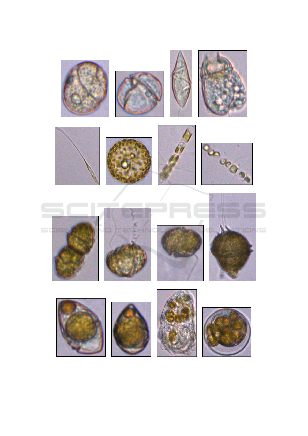
an image classiﬁcation problem. Figure 1 shows some

examples of zooplankton, phytoplankton and zoo-

plankton consuming phytoplankton. Since each im-

age of the dataset must contain a single organism and

were obtained cropping the collates formed by the mi-

croscopy, their resolution is not homogeneous, vary-

ing with the type, size and form of each individual.

For instance, resolutions of images of Figure 1-(a) to

(d) were, respectively, 138 × 160, 119 × 112, 82 ×

248, and 139 × 190 pixels, and resolutions of images

of Figure 1-(e) to (h) were, respectively, 295 × 388,

189 × 192, 134 × 215, and 168 × 138 pixels.

This dataset was used to re-train, validate and test

an EfﬁcientNetv2 B3 (Tan and Le, 2019) pre-trained

model obtained from the Tensor Flow Hub (Tensor-

Flow-Org, 2023). Image resolution required a pre-

adjustment to 300 × 300 pixels. EfﬁcientNet is one of

the most powerful Convolutional Neural Network ar-

chitectures available online, used worldwide to clas-

sify images in numerous relevant applications with

excellent results (de Zarz

a et al., 2022) (Huang and

Liao, 2023). Images containing either PHY, ZOO

or ZCP were clustered in 3 completely disjointed

groups: Training, Validation and Test, each account-

ing for 40, 10 and 50% of the whole image set, and

distributed as shown in Table 1. The Training and Val-

idation groups were used to re-conﬁgure and re-train

the EfﬁcientNetv2 B3 model, and the Test group was

used to evaluate the performance of the resulting re-

trained structure with a set of images not involved in

the training phase. All aforementioned images were

manually classiﬁed to generate a ground truth needed

for both phases, training and testing: manual classiﬁ-

cations are needed for the Neural Network to learn the

speciﬁc weights and biases of the model, and to quan-

tify the trained model performance comparing each

predicted clustering with the corresponding ground

truth. During the testing phase, the outputs of the

trained model were visually identiﬁed as True Pos-

itive (TP), True Negative (TN), False Positive (FP),

and False Negative (FN) to compute the following

metrics:

Precision =

T P

(T P + FP)

Recall =

T P

(T P + FN)

F1 − score =

(2 ∗ precision ∗ recall)

(precision + recall)

Accuracy =

(T P + T N)

(T P + T N + FP + FN)

VISAPP 2024 - 19th International Conference on Computer Vision Theory and Applications

608

(a) (b) (c) (d)

(e) (f) (g) (h)

(i) (j) (k) (l)

(m) (n) (o) (p)

Figure 1: Samples of zooplankton ((a)-(d)), phytoplankton ((e)-(l)) and zooplankton consuming phytoplankton ((m)-(p)),

included in the ﬁrst dataset. (e)-(h) are diatoms, singles ((e) and (f)) and forming chains ((g) and (h)). (i)-(l) are dinoﬂagellates.

Microplankton Discrimination in FlowCAM Images Using Deep Learning

609

Table 1: Number of images of each microplankton type

used to train, validate, and test the EfﬁcientNetv2 B3 net-

work.

Training Validation Test Total

ZCP 180 44 224 448

ZOO 112 28 139 279

PHY 585 146 730 1461

Total 877 218 1093 2188

2.6 Object Detection: Identifying

Multiple Cells in an Image

One of the challenges with identifying and deter-

mining phytoplankton abundance is the ability of di-

noﬂagellates and diatoms, two distinct types of phyto-

plankton, to form chains. This complicates the identi-

ﬁcation of different species and also makes it difﬁcult

to count the total number of individuals using just im-

age classiﬁcation. Figures 1-(g)-(h) shows some sam-

ples of diatom chains from natural samples.

This second stage centers on phytoplankton and

approaches an object classiﬁcation problem rather

than an image classiﬁcation one. Now, the prob-

lem is solved using the fourth version of Ultralitics

You Only Look Once (YOLO) software infrastructure

(Bochkovskiy et al., 2020). YOLO is an open source

software package that implements deep learning and

neural networks, easy, efﬁcient and proven to perform

excellently in object detection and image segmenta-

tion in multiple environments (Diwan et al., 2023)

(Lee and Hwang, 2022).

More than 5000 color images were manually la-

beled and clustered into 3 classes: Dinoﬂagellates,

Diatoms and Chlamydomonas. Dinoﬂagellates and

diatoms from natural sampling and used in the phy-

toplankton images of the previous dataset were sep-

arated. Monoculture images of P. tricornutum were

added to the images of diatoms from natural samples,

and monoculture images of A. minutum were added

to the images of dinoﬂagellates from natural samples.

As C. reinhardtii is a freshwater algae and not found

in marine environments, it was kept in its own class.

Labeled images were also split in 3 different groups:

Training, Validation and Testing. The ground truth

consists of bounding boxes framing each individual

of each class found in each image. These bounding

boxes found in the Training and Validation images are

the elements used by the network to learn the internal

weights and biases, instead of the whole images. The

resolution of all these images was ﬁxed to 416 × 416

pixels.

Table 2 shows the number of images and individu-

als of different classes visually identiﬁed in the image

set. The last column shows the average number of in-

dividuals per class and per image. Table 3 shows the

distribution of the individuals of different classes in

the three subsets for training, validation and testing.

Original and hand-labeled Testing images were in-

put in the trained model to assess its performance,

using Precision, Recall, Accuracy, and F1-score, as

deﬁned in section 2.5. In object detection, the In-

tersection over Union (IoU) is deﬁned as the area of

the intersection of two bounding boxes over that of

their union. A common strategy to evaluate object

detectors, such as YOLO v4 in this case, is to select

the bounding boxes predicted by the trained model

whose detection score exceed a predeﬁned threshold

α. Each bounding box output by the network is as-

sociated with the ground truth bounding box of the

same image that has a maximum IoU, if that IoU

exceeds a certain threshold β. The number of True

Positives (TP) are the predicted bounding boxes that

have been associated with a ground truth bounding

box, the False Positives (FP) are the predicted bound-

ing boxes that have not been associated to any ground

truth bounding box, and the False Negatives (FN) are

the ground truth bounding boxes not associated to any

prediction (Padilla et al., 2020). The Precision-Recall

Curve is built by computing these metrics for differ-

ent β values. Then, the pairs of obtained Precisions

and Recalls are sorted by the Recall value and plot-

ted. The area below this Precision-Recall Curve will

range from 0 to 1, and it is called the Average Pre-

cision (AP). A perfect object detector generates AP

close to 1, and random object detectors result in a AP

around 0.5. The mAP can be deﬁned as the average of

AP, for the different classes. A common approach is

to use β = 0.5 (AP@0.5) as a good indicator of detec-

tion ability. According to several approaches widely

used in Deep Learning, AP and mAP correspond to

the same calculation (Wood and Chollet, 2022).

Trainings and Validations were performed under

a Google Colaboratory (Google, 2023) environment

using a GPU. Colaboratory is a hosted Jupyter Note-

book service with no setup required, and ready to use.

It provides free access to Machine and Deep learning

computing resources, including GPUs and TPUs.

3 EXPERIMENTAL RESULTS

This section gives the ﬁrst results obtained in two

fronts: 1) the assessment of the image classiﬁcation

network used to distinguish among different types of

plankton (PHY, ZOO and ZCP), and 2) the evaluation

of the object detector model to discriminate among

different types of phytoplankton.

VISAPP 2024 - 19th International Conference on Computer Vision Theory and Applications

610

Table 2: Number of individuals identiﬁed in all the images used to train the object detection network.

Class Number of Images Total Number of Individuals Individuals per image

Chlamydomonas 1520 1666 1.10

Dinoﬂagellates 2940 3148 1.07

Diatoms 785 2302 2.93

Total 5245 7116 1.35

Table 3: Number of individuals of each class used to train,

validate, and test the YOLO network.

Class Train Validation Test

Chlamydomonas 595 458 467

Dinoﬂagellates 1179 880 881

Diatoms 324 235 226

Total 2098 1573 1574

Table 4: Evaluation metrics for image classiﬁcation.

Class Accuracy Precision Recall F1-Score

PHY 97.43% 99.29% 96.84% 98.05%

ZCP 96.43% 87.14% 96.87% 91.75%

ZOO 98.07% 94.73% 90.00% 92.30%

3.1 Image Classiﬁcation

Table 4 shows the scores of the different metrics

used to assess the performance of the image classi-

ﬁer model. Accuracy, Precision and Recall surpass all

the 90%, except the Precision in the detection of ZCP,

which is greater than 87%. Accordingly, F1-Scores

are all > 90%. All these results were obtained from

the Testing dataset.

3.2 Object Detection

Table 5 shows the value of the Average Precision with

the IoU threshold β ﬁxed in 0.5 (AP@0.5) for the

three different types of phytoplankton. The Mean Av-

erage Precision computed as the mean of all the AP

values included in table 5 is mAP(0.5)= 97.47%, a

reference value that indicates a high performance of

the trained object classiﬁer.

Figure 2 shows several samples of inferences out-

put by the trained model.

Four diatoms at the top, in the middle, four di-

noﬂagellates and at the bottom, four images with C.

reinhardtii. Notice how, in the images of diatoms that

form chains, each element of the chain is marked sep-

arately as one inference of one diatom, although all

diatoms inferred in the image form a larger biological

structure.

Table 5: Average Precision per class with a β=0.5.

Class Dinoﬂagelates Diatoms Chlamy.

AP(0.5) 99.70% 99.60% 93.10%

4 CONCLUSIONS

This paper advances automatic classiﬁcation of dif-

ferent species of plankton viewed in images recorded

using a FlowCAM. Our approach is based on train-

ing CNNs using an extensive and widely assorted im-

age set obtained from ﬁeld samples collected at a lo-

cal beach in Mallorca and supplemented with images

from monocultures to identify zooplankton and phy-

toplankton, and to identify different individuals of

phytoplankton in a single image. The system, once

trained, is a potential solution to separate and taxo-

nomically identify plankton in the thousands of im-

ages which can be potentially recorded from micro-

scopic imaging methods, avoiding tedious, slow, and

sometimes imprecise manual identiﬁcation and label-

ing.

The work has been divided in two parts: ﬁrstly, an

image classiﬁcation network trained with a structure

based on EfﬁcientNetv2 B3, focused on distinguish-

ing images that contain either phytoplankton or zoo-

plankton; and secondly, a YOLO v4 object classiﬁca-

tion model trained to discriminate different types of

phytoplankton. In the ﬁrst case, more than 2000 im-

ages were used to train the system, and in the second

case, more than 7000 individuals of different species

from more than 5000 images were input in the YOLO

v4 network to be trained, validated and tested. All

images involved in both parts were carefully hand-

labeled to build the ground truth. The preliminary re-

sults show how well the classiﬁcation succeeds with

both models, reaching, in the ﬁrst one, 90% in terms

of F1-Score, and > 93% of Average Precision with a

IoU of 0.5 in the second one.

These results encourage the authors of this pa-

per to extend the work in several directions. Ongo-

ing work is centered on the analysis of results with

a wider range of IoU thresholds. However, there

are other points that deserve our attention and could

also be included in the forthcoming work. Metrics

of Precision, Recall, Fall-out and Accuracy need to

be analyzed for the different classes of phytoplank-

ton, so that further and more solid conclusions about

the classiﬁer performance can be inferred, and see

if the model needs to be re-trained with more or

different images. Additionally, the image database

Microplankton Discrimination in FlowCAM Images Using Deep Learning

611

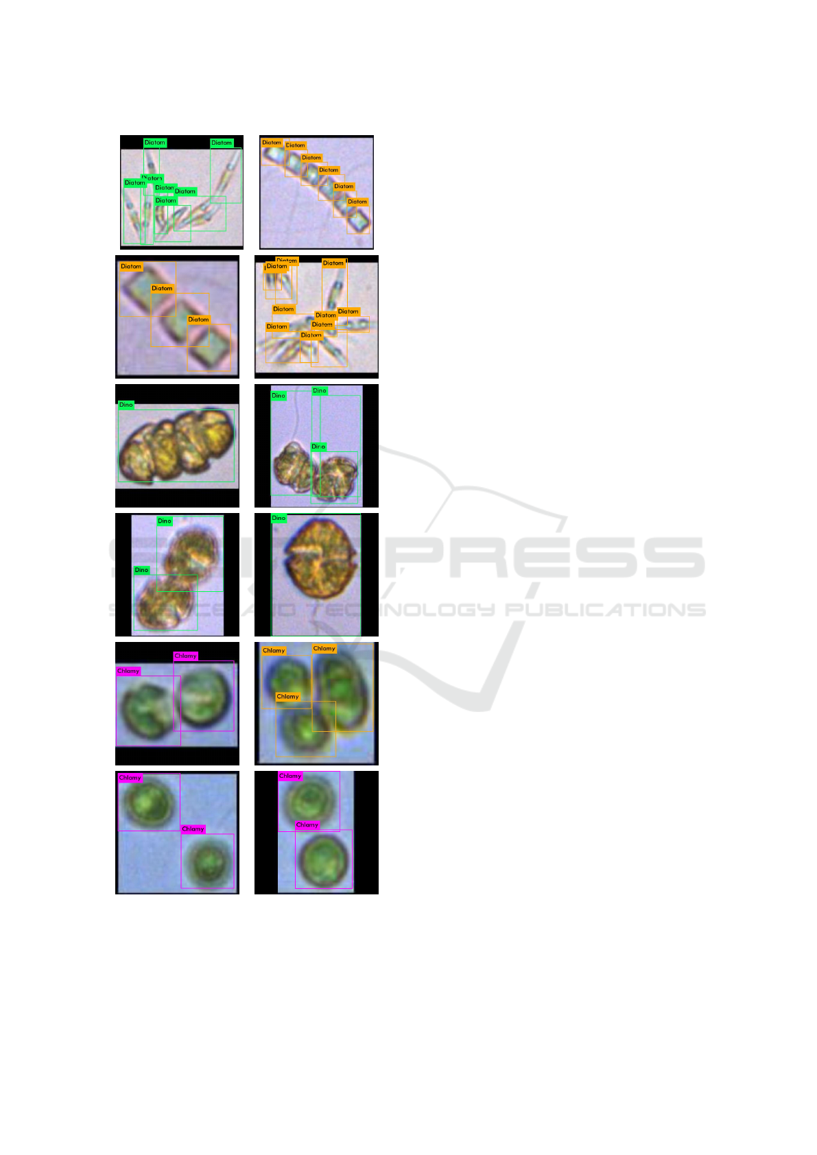
Figure 2: Sample inferences output by the YOLO model.

used to build the different train, validation and test-

ing datasets can be expanded with other samples col-

lected in different areas of the Balearic shoreline and

globally to increase and expand the detection of other

individuals of other types of plankton organisms. Fur-

thermore, more advanced network infrastructures can

be tested, such as the 3 different versions of YOLO

v8, the small, the medium and the large; usually, the

greater is the size of the trained model, the ﬁnest is its

performance; however, larger models entail more pro-

cessing power. Testing different sizes of trained clas-

siﬁers will permit us to ﬁnd the compromise between

desired or needed detection quality and the available

computational resources. All in all, this work has

demonstrated the power of the Deep Learning infras-

tructures to ease and automate the analysis and pro-

cessing of thousands of images which are obtained

from Imaging Microscopy machines like the Flow-

CAM, and the absolute feasibility for this type of bi-

ological applications of CNNs.

ACKNOWLEDGEMENTS

The authors thank Raquel Guti

erez Cuenca, Paula Is-

abel Gonzalo Valmala, Alba G

omez Rubio, Benjam

ın

Casas, and both current and past members of the In-

FiBio group for their support collecting and process-

ing water samples from Cala Santany

ı.

REFERENCES

Alzubaidi, L., Zhang, J., Humaidi, A., Al-Dujaili, A., Duan,

Y., Al-Shamma, O., Santamar

ıa, J., Fadhel, M., Al-

Amidie, M., and Farhan., L. (2021). Review of Deep

Learning: Concepts, CNN Architectures, Challenges,

Applications, Future directions. Journal of Big Data,

8(53):12853–12884.

Basterretxea, G., Garc

e, E., Jordi, A., and Mas

o, M. (2007).

Modulation of Nearshore Harmful Algal Blooms by in

situ Grouth Rate and Water Renewal. Marine Ecology

Progress Series, 352:53–65.

Basterretxea, G., Tovar-S

anchez, A., Beck, A. J., Masqu

P., Bokuniewicz, H. J., Coffey, R., Duarte, C. M.,

Garcia-Orellana, J., Garcia-Solsona, E., Martinez-

Ribes, L., and Vaquer-Sunyer, R. (2010). Submarine

Groudwater Discharge to the Coastal Environment of

a Mediterranean Island. Ecosystem and Biogeochemi-

cal Signiﬁcance. Ecosystems, 13:629–643.

Bochkovskiy, A., Wang, C.-Y., and Liao, H.-Y. M.

(2020). Yolov4: Optimal Speed and Accuracy

of Object Detection. https://github.com/ultralytics/,

https://arxiv.org/abs/2004.10934.

Buskey, E. J. and Hyatt, C. J. (2006). Use of the FlowCAM

for Semi-automated Recognition and Enumeration of

VISAPP 2024 - 19th International Conference on Computer Vision Theory and Applications

612

Red Tide Cells (Karenia brevis) in Natural Plankton

Simples. Harmful Algae, 5(6):685–692.

de Zarz

a, I., de Curt

o, J., and Calafate, C. T. (2022). De-

tection of Glaucoma using Three-stage Training with

EfﬁcientNet. Intelligent Systems with Applications,

16:200140.

Diwan, T., Anirudh, G., and Tembhurne, J. V. (2023). Ob-

ject Detection using YOLO: Challenges, Architectural

Successors, Datasets and Applications. Multimedia

Tools and Applications, 82(6):9243–9275.

Dubelaar, G. B. and Jonker, R. R. (2000). Flow Cytometry

as a Tool for the Study of Phytoplankton. Scientia

Marina, 64(2):135–156.

Figueroa, R., Garc

es, E., Massana, R., and Camp, J. (2008).

Description, Host-speciﬁcity and Strain Selectivity of

the Dinoﬂagellate Parasite Parvilucifera sinerae sp.

Nov. (Perkinsozoa). Protist, 159(4):563–578.

Fuchs, R., Thyssen, M., Creach, V., Dugenne, M., Izard,

L., Latimier, M., Louchart, A., Marrec, P., Rijkeboer,

M., Gr

egori, G., et al. (2022). Automatic Recognition

of Flow Cytometric Phytoplankton Functional Groups

using Convolutional Neural Networks. Limnology and

Oceanography: Methods, 20(7):387–399.

Google (2023). Google Colaboratory: a Hosted Jupyter

Notebook Service. https://colab.google/.

Henrichs, D., Angl

es, S., Gaonkar, C., and Campbell, L.

(2021). Application of a Convolutional Neural Net-

work to Improve Automated Early Warning of Harm-

ful Algal Blooms. Environmental Science and Pollu-

tion Research, 28:28544–28555.

Huang, M.-L. and Liao, Y.-C. (2023). Stacking Ensem-

ble and ECA-EfﬁcientNetV2 Convolutional Neural

Networks on Classiﬁcation of Multiple Chest Dis-

eases Including COVID-19. Academic Radiology,

30(9):1915–1935.

Hussain, M., Bird, J. J., and Faria, D. R. (2019). A Study

on CNN Transfer Learning for Image Classiﬁcation.

In Advances in Computational Intelligence Systems,

pages 191–202.

Kerr, T., Clark, J. R., Fileman, E. S., Widdicombe, C. E.,

and Pugeault, N. (2020). Collaborative Deep Learn-

ing Models to Handle Class Imbalance in FlowCam

Plankton Imagery. IEEE Access, 8:170013–170032.

Lee, J. and Hwang, K.-i. (2022). YOLO with Adap-

tive Frame Control for Real-time Object Detection

Applications. Multimedia Tools and Applications,

81(25):36375–36396.

Menden-Deuer, S., Morison, F., Montalbano, A. L., Franz

G., Strock, J., Rubin, E., McNair, H., Mouw, C.,

and Marrec, P. (2020). Multi-Instrument Assess-

ment of Phytoplankton Abundance and Cell Sizes in

Mono-Speciﬁc Laboratory Cultures and Whole Plank-

ton Community Composition in the North Atlantic.

Frontiers in Marine Sciences, 7(254).

Padilla, R., Netto, S. L., and da Silva, E. A. B. (2020). A

Survey on Performance Metrics for Object-Detection

Algorithms. In Proceedings of the International Con-

ference on Systems, Signals and Image Processing

(IWSSIP), pages 237–242.

Rodellas, V., Garcia-Orellana, J., Masqu

e, P., and Wein-

stein, Y. (2015). Submarine Groundwater Discharge

as a Major Source of Nutrients to the Mediterranean

Sea. The Proceedings of the National Academy of Sci-

encese PNAS, 112(13):3926–3930.

Sosa-Trejo, D., Bandera, A., Gonz

alez, M., and Hern

andez-

on, S. (2023). Vision-based Techniques for Auto-

matic Marine Plankton Classiﬁcation. Artiﬁcial Intel-

ligence Reviews, 56:12853–12884.

Tan, M. and Le, Q. (2019). EfﬁcientNet: Rethinking Model

Scaling for Convolutional Neural Networks. In Pro-

ceedings of the 36th International Conference on Ma-

chine Learning, pages 6105–6114.

Tensor-Flow-Org (2023). Tensor Flow Hub, a Repos-

itory of Trained Machine Learning Models.

https://www.tensorﬂow.org/hub.

Tovar-S

anchez, A., Basterretxea, G., Rodellas, V., S

anchez-

Quiles, D., Garc

ıa-Orellana, J., Masqu

e, P., Jordi, A.,

opez, J. M., and Garcia-Solsona, E. (2014). Contri-

bution of Groundwater Discharge to the Coastal Dis-

solved Nutrients and Trace Metal Concentrations in

Majorca Island: Karstic vs. Detrital Systems. Environ

Sci. Technol, 48:11819–11827.

Ullah, I., Carri

on-Ojeda, D., Escalera, S., Guyon, I. M.,

Huisman, M., Mohr, F., van Rijn, J. N., Sun, H., Van-

schoren, J., and Vu, P. A. (2022). Meta-Album: Multi-

domain Meta-Dataset for Few-Shot Image Classiﬁca-

tion. In Neural Information Processing Systems.

Wood, L. and Chollet, F. (2022). Efﬁcient Graph-Friendly

COCO Metric Computation for Train-Time Model

Evaluation. https://arxiv.org/abs/2207.12120.

Yamazaki, H. (2022). Plankton Image Dataset from a Ca-

bled Observatory System (JEDI System/OCEANS)

Deployed at Coastal Area of Oshima Island, Tokyo,

Japan. https://doi.org/10.48518/00014.

Yokogawa (2023). FlowCam: Flow Imaging Microscopy.

https://www.yokogawa.com/solutions/products-

and-services/life-science/ﬂowcam-ﬂow-imaging-

microscopy/.

Zhang, J., Li, C., Yin, Y., Zhang, J., and Grzegorzek, M.

(2023). Applications of Artiﬁcial Neural Networks

in Microorganism Image Analisis: a Comprehensive

Review from Conventional Multilayer Perceptron to

Popular Convolutional Neural Network and Potential

Visual Transformer. Artiﬁcial Intelligence Review,

56:1013–1070.

Zhang, Y., Lu, Y., Wang, H., Chen, P., and Liang, R.

(2021). Automatic Classiﬁcation of Marine Plankton

with Digital Holography Using Convolutional Neural

Network. Optics and Laser Technology, 139:106979.

Zingone, A., Escalera, L., Aligizaki, K., Fern

andez-Tejedor,

M., Ismael, A., Montresor, M., Mozeti

c, P., Tas¸, S.,

and Totti, C. (2021). Toxic Marine Microalgae and

Noxious Blooms in the Mediterranean Sea: A Con-

tribution to the Global HAB Status Report. Harmful

Algae, 102:101843.

Microplankton Discrimination in FlowCAM Images Using Deep Learning

613