Anomaly Detection on Roads Using an LSTM and Normal Maps

Yusuke Nonaka

1 a

, Hideo Saito

1 b

, Hideaki Uchiyama

1 c

, Kyota Higa

and Masahiro Yamaguchi

Keio University, Yokohama, Japan

NEC Corporation, Kawasaki, Japan

Keywords:

Deference-in-Level Detection, Unsupervised Learning, Outdoor Navigation, Anomaly Detection.

Abstract:

Detecting anomalies on the road is crucial for generating hazard maps within factory premises and facilitating

navigation for visually impaired individuals or robots. This paper proposes a method for anomaly detection on

road surfaces using normal maps and a Long Short-Term Memory (LSTM). While existing research primarily

focuses on detecting anomalies on the road based on variations in height or color information of images, our

approach leverages anomaly detection to identify changes in the spatial structure of the walking scenario.

The normal (non-anomaly) data consists of time series normal maps depicting previously traversed roads,

which are utilized to predict the upcoming road conditions. Subsequently, an anomaly score is computed by

comparing the predicted normal map with the normal map at t +1. If the anomaly score exceeds a dynamically

set threshold, it indicates the presence of anomalies on the road. The proposed method employs unsupervised

learning for anomaly detection. To assess the effectiveness of the proposed method, we conducted accuracy

assessments using a custom dataset, taking into account a qualitative comparison with the results of existing

methods. The results conﬁrm that the proposed method effectively detects anomalies on road surfaces through

anomaly detection.

1 INTRODUCTION

Among technologies for detecting anomalies on

roads, difference-in-level detection technology has

signiﬁcant potential applications, including aiding vi-

sually impaired individuals and the elderly in walking

and generating hazard maps in factory environments.

However, while there has been considerable research

on curb detection and bump detection for road appli-

cations in the ﬁeld of automated driving, there is a

limited amount of research focused on detecting vari-

ous types of outdoor differences in road levels.

Several methods have been proposed for detect-

ing differences in level. Imai et al. (K. Imai et al.,

2017) presented a method that utilizes an RGB-D

camera to identify walkable planes, considering the

difference in height between detected planes as dif-

ferences in road level. Yanagihara et al. (K. Yanag-

ihara et al., 2020) employed a Convolutional Neural

Network (CNN) and Grad-weighted Class Activation

Mapping (Grad-CAM)(R.R. Selvaraju et al., 2017) to

detect differences in road levels. This approach vi-

https://orcid.org/0000-0002-9180-6020

https://orcid.org/0000-0002-2421-9862

https://orcid.org/0000-0002-6119-1184

sualizes the decision-making process of the CNN in

classifying RGB images with and without differences

in level. Nonaka et al.(Y. Nonaka et al., 2023) divided

images into small patches and employed a CNN to

classify these patches into three categories, including

a “difference-in-level” class. The CNN model was

used to classify and detect patches belonging to the

difference-in-level class.

However, all of these methods deﬁne the differ-

ence in level solely based on difference in height,

without considering the potential hazard level based

on the surrounding environment. For instance, a haz-

ardous situation arises when the user perceives the

upcoming area as walkable based on visual informa-

tion, but encounters unexpected differences in level

on road. In essence, a difference in level can be iden-

tiﬁed when the user attempts to traverse a plane that

deviates from the expected plane, irrespective of its

vertical elevation.

Furthermore, in the context of anomaly detection

on roads in autonomous driving, there exist meth-

ods that are applicable to walking scenarios. As

one example of such methods, Voj

r et al.(T. Voj

and J. Matas, 2023) uses only RGB images as input,

identifying the entire non-road region as an anomaly.

244

Nonaka, Y., Saito, H., Uchiyama, H., Higa, K. and Yamaguchi, M.

Anomaly Detection on Roads Using an LSTM and Normal Maps.

DOI: 10.5220/0012458900003660

Paper published under CC license (CC BY-NC-ND 4.0)

In Proceedings of the 19th International Joint Conference on Computer Vision, Imaging and Computer Graphics Theory and Applications (VISIGRAPP 2024) - Volume 2: VISAPP, pages

244-255

ISBN: 978-989-758-679-8; ISSN: 2184-4321

The method leverages a signiﬁcant increase in er-

rors speciﬁcally within the anomaly-containing area

by comparing the inpainted image of the region es-

timated to contain anomalies with the input image.

This enables the identiﬁcation of regions with anoma-

lies. Nevertheless, since this method relies solely on

RGB images, it is not effective when the color of

anomalous objects is similar to that of the road region

in the images.

The purpose of this paper is to detect anoma-

lies that occur when the anticipated continuity of

the current walking plane is disrupted by unexpected

changes. In this paper, ”unexpected changes” refer

to variations in walking surface conditions, such as

transitioning from a gravel path to a grassy area, and

the emergence of anomalies that are not visually per-

ceivable from color information, such as objects with

colors similar to the road surface. The aforemen-

tioned existing methods detect anomalies based on

color information in images or the height of anoma-

lies from the walking plane, making it challenging

to detect all anomalies caused by the deﬁned ”un-

expected changes” that are likely to lead to falls in

walking scenarios. The proposed approach predicts

the normal map of the walking surface to be tra-

versed based on past time-series normal maps. It

then computes an anomaly score by comparing the

predicted normal map with the normal map at t + 1

and determines the presence of anomalies when the

anomaly score surpasses a dynamically set threshold.

To achieve this, the prediction involves using a Long

Short-Term Memory (LSTM), but the normal maps

are transformed into a feature vector using a Varia-

tional Autoencoder (VAE), which serves as the input

for an LSTM. This method allows for the detection of

anomalies caused by ”unexpected changes” by rely-

ing solely on the information from the past few frames

of normal maps, without utilizing color information

even when walking on unknown surfaces.

To evaluate the effectiveness of the proposed

method, we constructed a custom dataset and con-

ducted quantitative and qualitative evaluations, com-

paring the results with those of an existing method for

anomaly detection. As a result, the proposed method

demonstrated its efﬁcacy as the ﬁrst approach to de-

tect anomalies and surface changes unpredictably ap-

pearing on the road using anomaly detection. In sum-

mary, the contributions of the proposed method are as

follows:

• A new approach to detecting changes in walking

surface conditions without relying on labeled data

for unknown anomalies.

• Enhanced robustness to noise by incorporating a

VAE, compared to a straightforward use of normal

maps as LSTM inputs.

• Successful implementation of a dynamic thresh-

old, alerting at the moment when the road surface

undergoes a change.

2 RELATED WORK

2.1 Anomaly Detection on Roads

Among the latest studies on road anomaly detection, a

notable mention is (T. Voj

r and J. Matas, 2023) which

presents a methodology applicable to walking scenar-

ios without constraints on road types. This study fo-

cuses on the difﬁculty in inpainting anomalies in RGB

images. It acknowledges the challenge of inpainting

anomalies in RGB images because anomalies often

differ from the surrounding color information. The

methodology leverages only RGB images as input,

capable of detecting anomalies on various road sur-

faces, recognizing anomalies present on the road sur-

face regardless of the surface type. However, its effec-

tiveness diminishes when the colors of the road sur-

face and anomalies are similar in the RGB images. In

walking scenarios, detecting anomalies in such con-

ditions becomes crucial.

2.2 Difference-in-Level Detection

Detecting differences in level remains a challenging

task, especially when considering the wide range of

variations in outdoor environments. To illustrate an

instance of difference-in-level detection for the visu-

ally impaired, Imai et al. (K. Imai et al., 2017) intro-

duced a method that utilizes an accelerometer and a

depth camera to detect ﬂat surfaces and identify dif-

ferences in level on road. In this method, the ﬁrst step

involves measuring the distance between the measur-

ing device and the user’s feet, which is then set as

the reference height for the current walking surface.

Next, the method identiﬁes points from the acquired

point clouds that have normal vectors parallel to the

normal vector of the current walking plane. Subse-

quently, the vertical height of these extracted points is

measured and compared to the ﬁxed reference height.

If the height difference exceeds a threshold, the point

is determined to be a part of the difference in level on

the current walking plane.

Yanagihara et al. (K. Yanagihara et al., 2020) pro-

posed a method using a combination of CNN and

Grad-CAM. The method employs RGB images and

CNNs, where a CNN model is trained to classify road

images into two categories: those with differences

Anomaly Detection on Roads Using an LSTM and Normal Maps

245

in level and those without. To gain insights into the

decision-making process of the CNN model, Grad-

CAM visualization is utilized, providing a visual in-

terpretation of the basis for the model’s classiﬁca-

tions.

Nonaka et al. (Y. Nonaka et al., 2023) employed a

method where the image is divided into small patches,

and a CNN is used to classify these patches into one

of three classes. Among these classes, one class is

the difference-in-level class, and the center pixel of

an image patch belonging to this class is identiﬁed

as having a difference in level. By passing all the

image patches obtained from the image through the

CNN model and classifying them, differences in level

on road within the image can be detected.

In all of the aforementioned methods, the primary

focus lies in detecting the location of differences in

level within the images. However, these approaches

do not speciﬁcally address the level of danger associ-

ated with the identiﬁed differences in level on road.

2.3 Forecasting-Based Time Series

Anomaly Detection

According to the deﬁnition provided in (Z. Z. Dar-

ban et al., 2022), deep anomaly detection in time

series can be classiﬁed into two main approaches:

forecasting-based and reconstruction-based. Each ap-

proach can further be categorized into different sub-

categories based on the model architecture employed.

In this subsection, we will focus on the forecasting-

based methods and speciﬁcally discuss related works

that utilize Recurrent Neural Networks (RNN) with

multidimensional input data, similar to the approach

proposed in our method.

DeepLSTM (S. Hochreiter and J. Schmidhuber,

2015) employs stacked LSTM recurrent networks to

train on normal time series data. The model ﬁts the

prediction error vectors to a multivariate Gaussian

distribution using maximum likelihood estimation.

By predicting a mixture of anomaly and normal data,

the model records the Probability Density Function

(PDF) values associated with the prediction errors.

In LSTM-NDT (K. Hundman et al., 2018), a com-

bination of techniques including LSTM and RNN is

utilized to achieve accurate predictions by leveraging

historical information from multivariate time series.

The paper introduces a dynamic unsupervised thresh-

olding method for evaluating residuals, enabling auto-

matic thresholding for evolving data. This approach

addresses the challenges posed by diversity, instabil-

ity, and noise in the data.

However, none of the forecasting-based methods

utilizing RNNs, including the aforementioned stud-

Past Walked-on

Road Surface

Future Walking

Road Surface

Past Walked-on

Road Surface

Future Walking

Road Surface

Detection of an anomaly object

Detection of road surface change

Figure 1: Illustration of anomaly detection in this study:

The left illustration represents the case of detecting anomaly

objects. The right illustration represents the case of detect-

ing anomalies when there is a change in the road surface

condition.

ies (J. Goh et al., 2017; N. Ding et al., 2019; L. Shen

et al., 2020; W. Wu et al., 2020), have employed nor-

mal maps as input.

3 PROPOSED METHOD

3.1 Overview

The objective of this study is to develop a system ca-

pable of detecting hazardous differences in level on

roads, even when the user perceives no difference

based on visual information but ends up falling. To

achieve this, the proposed method employs normal

maps as input instead of RGB images. By utilizing

normal maps, the method aims to detect differences in

level that may be overlooked by relying solely on vi-

sual information. The normal maps utilized in this pa-

per are generated using the technique described in (Y.

Nonaka et al., 2023).

As depicted in Figure 1, to prevent the risk of

falls, it is crucial to detect the presence of a surface

condition different from the current walking plane in

the plane intended for walking. Therefore, the con-

ﬁguration involves combining an LSTM for predict-

ing the plane condition intended for walking and a

VAE for maintaining spatial information in the input

to the LSTM while utilizing normal maps. As a re-

sult, the network architecture of the proposed method

becomes as depicted in Figure 2.

In this approach, the input normal maps undergo

compression into low-dimensional vectors using the

encoder of the VAE. Subsequently, by using the time-

series feature vectors as input for the LSTM, the

LSTM outputs a predicted feature vector of a nor-

mal map at t + 1, and the normal map at t + 1 is

transformed into a low-dimensional vector by the pre-

trained VAE’s encoder. Finally, the anomaly score

is computed as the prediction error between the pre-

dicted normal map and the normal map at t + 1 using

VISAPP 2024 - 19th International Conference on Computer Vision Theory and Applications

246

Encoder

t+1

LSTM

Input: time series normal maps

time series feature vectors

Normal map compression

Next-frame prediction

normal map

at t+1

predicted

feature vector

at t+1

Difference-in-level detection

using anomaly detection

input

output

Encoder

t+1

feature vector

at t+1

Anomaly

Score

MSE

Figure 2: Overview of the proposed method. The leftmost images represent time series normal maps, which are transformed

into low-dimensional feature vectors by the encoder of a pre-trained Variational Autoencoder (VAE). These vectors become

inputs to a Long Short-Term Memory (LSTM). The output of the LSTM generates a low-dimensional feature vector for a

predicted frame. The rightmost normal map at t + 1 corresponds to the normal map derived from a depth image captured by a

camera. The normal map is transformed into a low-dimensional vector by the encoder of a pre-trained VAE. Then, the feature

vectors of the predicted normal map at t + 1 and the normal map at t + 1 are compared, and the loss is computed with Mean

Squared Error (MSE).

Mean Squared Error (MSE). If the anomaly score ex-

ceeds a dynamically set threshold, the frame is classi-

ﬁed as an anomaly frame.

3.2 Compression of Normal Maps Using

a VAE

To preserve the spatial information of images when

using them as inputs for the LSTM, the proposed

method incorporates a VAE. The VAE is employed to

extract abstract and compressed features in the bottle-

neck layer located between the decoder and encoder.

Speciﬁcally, in this study, the β-VAE (I. Higgins et al.,

2016) is initially trained to reconstruct a normal map.

This training process generates an encoder, which

compresses the normal map into a low-dimensional

vector, and a decoder, which reconstructs the normal

map from the low-dimensional vector.

We employ a Convolutional Variational Autoen-

coder (ConvVAE) model for training, which is based

on the model used in (D. Ha and J. Schmidhuber,

2018). The VAE is trained by optimizing the Evi-

dence Lower Bound (ELBO), as deﬁned in (I. Hig-

gins et al., 2016). The ELBO comprises two terms:

the reconstruction error, which measures the discrep-

ancy between an input and its corresponding recon-

struction, and the Kullback-Leibler (KL) divergence,

which quantiﬁes the difference between the encoder

and decoder distributions. To compute the reconstruc-

tion error term in the ELBO, we employ the binary

cross entropy (BCE) loss function, which is deﬁned

as follows:

BCE = −

∑

n=1

∑

k=1

(1 − c

(k)

)log(1 − ˆc

(k)

) + c

(k)

log( ˆc

(k)

), (1)

where N is the size of mini-batch used in training,

D is the number of pixels, and the c

and ˆc

are the

ground-truth and reconstructed image’s pixel values,

which are normalized between 0 and 1, for the n

pixel respectively. In this paper, the BCE loss is not

divided by D in the VAE training.

3.3 Next-Frame Prediction by an LSTM

This section outlines the process of generating the

feature vector of the normal map at t + 1 using an

LSTM. The LSTM model is employed to generate fu-

ture images based on the given input sequence. We

utilizes time series normal maps of the previously tra-

versed road over the past several seconds as the ref-

erence normal (non-anomaly) data. Our approach in-

volves predicting a feature vector of a normal map for

the upcoming road segment and computing the pre-

diction error between the predicted feature vector and

a feature vector of the normal map at t + 1. During

the training of an LSTM, the prediction error serves

as the loss of the network, but during the anomaly

frame detection explained in Section 3.4, it is called

as the anomaly score.

Consider a time series denoted as

X = {x

(1)

(2)

,.. .,x

(l)

}, where each time step

(t)

∈ R

C,H,W

represents a normal map. Here, l

(where l > 1) represents the number of frames

in the time series of normal maps used as input.

In this paper, we utilize a VAE to compress each

normal map into a feature vector, which serves as

an abstract representation of the respective input

frame. Therefore, utilizing the encoding process of

the pre-trained VAE, the time series X is compressed

into Z = {z

(1)

(2)

,.. .,z

(l)

}, where each time step

(t)

∈ R

corresponds to a low-dimensional fea-

ture vector of a normal map, and m represents the

dimension of the low-dimensional feature vector.

The LSTM then processes the input and produces

an output in the form of a low-dimensional feature

vector of the next frame, with a dimension of m.

Anomaly Detection on Roads Using an LSTM and Normal Maps

247

3.4 Detection of Anomaly Frames by

Dynamic Thresholds

Once a predicted feature vector of a normal map ˆy

(t)

is generated for each step t, an anomaly score is cal-

culated as following:

(t)

∑

n=1

( ˆy

(t)

− y

(t)

)

, (2)

where y

(t)

= z

(t+1)

is the feature vector of the normal

map at t +1. Assuming that the predicted feature vec-

tor is generated based on past normal (non-anomaly)

data, the anomaly score between the predicted feature

vector of a normal map at t + 1 and the feature vector

of the normal map at t + 1 is expected to be minimal

if there are no anomalies.

The following describes the technique for dy-

namically setting thresholds and reducing false pos-

itives after calculating the anomaly score to deter-

mine whether a frame is anomalous. In this study, the

technique for dynamically setting the threshold and

reducing false positives in anomaly detection is em-

ployed based on the methods described in (K. Hund-

man et al., 2018).

Smoothing of Anomaly Scores. When an anomaly

score e

(t)

is calculated, each e

(t)

is appended to a one-

dimensional vector of anomaly scores:

e = [e

(t−h)

,.. .,e

(t−l)

,.. .,e

(t−1)

], (3)

where h is the number of historical anomaly scores

used to evaluate the current anomaly score. The

anomaly scores, denoted as e, undergo a smooth-

ing process to mitigate spikes commonly observed

in LSTM-based predictions. Sudden changes in

values are often imperfectly predicted, leading to

sharp spikes in error values, even in normal sce-

narios (D. T. Shipmon et al., 2017). We employ

an exponentially-weighted moving average (EWMA)

to produce the smoothed anomaly scores e

(t−h)

,.. .,e

(t−l)

,.. .,e

(t−1)

] (Hunter, 1986). Based

on the smoothed anomaly scores, a threshold is deter-

mined to classify whether the frame x

(t+1)

is normal

or anomalous. If the smoothed anomaly score e

(t)

ex-

ceeds the dynamically set threshold, it is determined

that there is an anomaly, speciﬁcally a difference in

level, in the next frame x

(t+1)

Dynamically Setting Thresholds. In this paper,

similar to (K. Hundman et al., 2018), we determine

a dynamic threshold for each predicted frame using

an unsupervised learning method that achieves high

performance with low overhead, without the need for

labeled data or statistical assumptions about anomaly

scores. Using a threshold ε chosen from the set:

ε = µ(e

) + zσ(e

) (4)

Where ε is determined by:

ε = argmax(ε

ε) =

∆µ(e

)/µ(e

) + ∆σ(e

)/σ(e

)

| + |E

seq

(5)

Such that:

∆µ(e

) = µ(e

) − µ({e

∈ e

< ε})

∆σ(e

) = σ(e

) − σ({e

∈ e

< ε})

= {e

∈ e

> ε}

seq

= continuous sequences of e

∈ e

The values used for evaluating ε are determined

by z ∈ z, where z is an ordered set of positive val-

ues representing the number of standard deviations

above µ(e

). After identifying argmax(ε

ε), a score s

is assigned to each resulting anomalous sequence of

smoothed anomaly scores e

seq

∈ E

seq

to indicate the

severity of the anomaly:

(i)

max(e

(i)

seq

) − argmax(ε

ε)

µ(e

) + σ(e

)

(6)

This involves ﬁnding a threshold where, if all val-

ues of e

above the threshold are removed, the mean

and standard deviation of the smoothed anomaly

scores e

would experience the greatest percent de-

crease. This function imposes penalties for an ex-

cessive greedy behavior, particularly when there are

larger numbers of anomalous values (|e

|) and se-

quences (|E

seq

|). Subsequently, each sequence of

anomalous errors assigns a normalized score to the

highest smoothed anomaly score based on its distance

from the chosen threshold.

False Positive Reduction. To reduce false posi-

tives, we introduce a pruning technique used in (K.

Hundman et al., 2018). This involves creating a

new set, e

max

, which includes max(e

seq

) for all e

seq

sorted in descending order. Additionally, we include

the maximum smoothed anomaly score that isn’t re-

garded as anomalous, max({e

∈ e

∈ E

seq

∋ e

}),

to the end of e

max

. The sequence is then itera-

tively processed, and the percentage decrease d

(i)

(i−1)

max

−e

(i)

max

)/e

(i−1)

max

at each step i is computed where

i ∈ {1, 2,... ,(|E

seq

| + 1)}. If, at a certain step i, d

(i)

exceeds a minimum percentage decrease p, a frame

with the anomaly score e

(i−1)

max

remain classiﬁed as an

anomaly frame, but if the percentage decrease falls

below p, it is reclassiﬁed as a normal (non-anomaly)

frame.

VISAPP 2024 - 19th International Conference on Computer Vision Theory and Applications

248

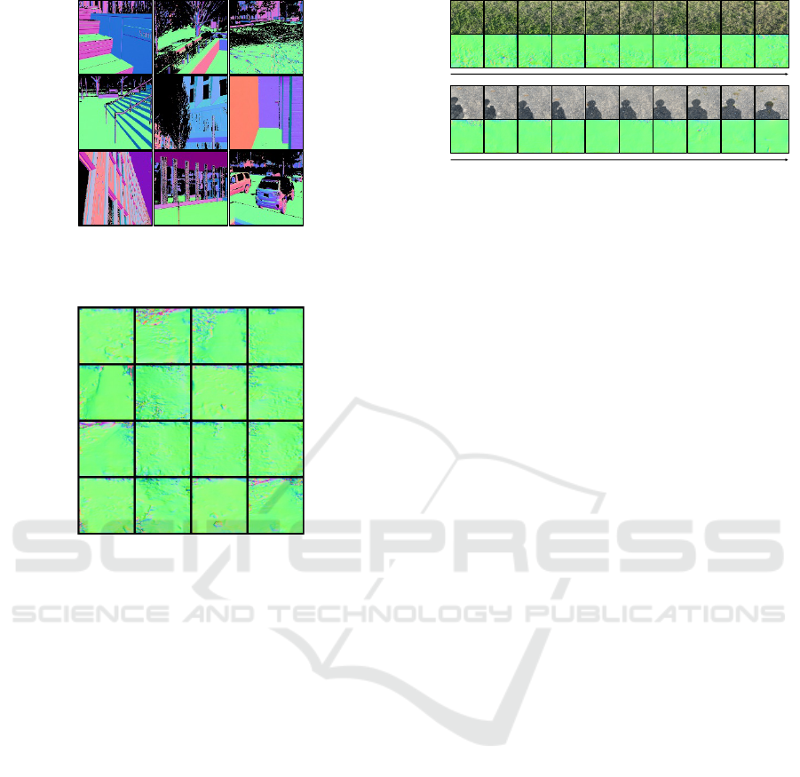
Figure 3: Examples of the normal maps in the Dense Indoor

and Outdoor DEpth (DIODE) (I. Vasiljevic et al., 2019)

dataset.

Figure 4: Examples of the normal maps used for ﬁne-tuning

the Variational Autoencoder (VAE) model.

4 EXPERIMENTS

4.1 VAE and LSTM Training

4.1.1 Overview

In this section, we describe the training of a VAE

and an LSTM used for anomaly detection. A VAE

was initially trained on normal maps from the pub-

licly available dataset, Dense Indoor and Outdoor

DEpth (DIODE) (I. Vasiljevic et al., 2019) and ﬁne-

tuned on our custom dataset. Subsequently, the pre-

trained VAE was utilized to train an LSTM on our

custom dataset. Details regarding the dataset used

are discussed in Section 4.1.2. Details on the net-

work training of the two models are provided in Sec-

tion 4.1.3. Results of the training are elaborated on in

Section 4.1.4.

4.1.2 Dataset

VAE. The VAE was pre-trained using the DIODE

dataset. The dataset consists of two scenes: outdoor

scenes (16,502 images in the training set) and indoor

RGB

Normal

𝒕

RGB

Normal

𝒕

Figure 5: Examples of the time series data utilized for train-

ing the Long Short-Term Memory (LSTM). The top row

corresponds to data from a grassy area, while the bottom

row represents data from a gravel path. Normal maps and

their corresponding RGB images are arranged chronologi-

cally. Although only the normal maps were employed as

training data, RGB images are also presented here to pro-

vide an overview of the dataset.

scenes (8,393 images in the training set), each with

corresponding normal maps. Figure 3 shows exam-

ples of normal maps included in the DIODE dataset.

We utilized training data from both scenes. Therefore,

the VAE model was trained on a dataset comprising

24,895 normal maps.

Subsequently, the pre-trained model was ﬁne-

tuned using our custom dataset, as illustrated in Fig-

ure 4, which includes normal maps of the ground

in scenes featuring grassy areas, asphalt, and gravel

roads. While the dataset comprises a total of 86

frames, it was divided into training (70 frames), vali-

dation (10 frames), and test (6 frames) sets. The nor-

mal maps used in our custom dataset were created

using depth images captured with an iPhone 12 Pro

Max.

LSTM. The LSTM was trained using a custom

dataset, as illustrated in Figure 5. The dataset com-

bines two scenes: one consists of time-series normal

maps of a grassy area, and the other comprises time-

series normal maps of a gravel road. The grassy area

exhibits irregularities on the normal maps, while the

normal maps of the gravel road show minimal irreg-

ularities. The dataset consists of 250 frames for the

grassy area’s time-series data and 40 frames for the

gravel road’s time-series data. In this paper, predict-

ing the feature vector of the next frame’s normal map

from a sequence of feature vectors of 5 consecutive

frames is accomplished using an LSTM. Therefore,

the total number of data points is 280. To create train-

ing, validation, and test set data, the dataset is divided

into training (210), validation (60), and test (10) data

points. Similar to the creation of the VAE’s custom

dataset, the normal maps used in the custom dataset

are captured using depth images from an iPhone 12

Pro Max. We used the camera on the smartphone to

capture 4 frames per second.

Anomaly Detection on Roads Using an LSTM and Normal Maps

249

4.1.3 Implementaion Detail

VAE. First, the settings during training using the

DIODE dataset is described. The dimension of the

VAE’s feature vector was set to 512, and the training

was conducted with a mini-batch size of 256. The net-

work optimizer used was Adam (D.P. Kingma and J.

Ba, 2015) with β

= 0.9 and β

= 0.999. The biases

of the convolutional layers were initialized to zero.

The learning rate was set to 0.001, and weight de-

cay was applied at 0.0001. The training process com-

prised 100 epochs, and no dropout was applied during

model training.

Next, the settings for the pre-trained VAE’s ﬁne-

tuning is described. The only difference in settings

from pre-training is that weight decay is 0.001, and

the mini-batch size is 5. Other hyperparameter values

for training remain the same as during pre-training.

During model training, we employed the early stop-

ping technique, where training is halted if no im-

provement in validation set loss is observed within

30 epochs. All experiments were implemented in Py-

Torch (v1.10.1) using Python 3.7.10 and executed on

an Nvidia GeForce GTX 1080 GPU with CUDA 10.1.

LSTM. The input time-series images, with a size

of 128 × 128, are initially compressed into 512-

dimensional vectors by the VAE and serve as input to

the LSTM. The output vector dimension of the LSTM

is 512, and this output becomes the feature vector of

the predicted normal map at t + 1.

The network optimization was performed using

Adam (D.P. Kingma and J. Ba, 2015), with β

= 0.9

and β

= 0.999, and a mini-batch size of 1. The biases

of the convolutional layers were initialized to zero.

The learning rate was set to 0.0001, and no weight

decay was applied. The training process consisted

of 200 epochs, and dropout was not utilized during

model training. The LSTM has 2 hidden layers. The

experiment was conducted in the same environment

as the VAE training, utilizing the previously men-

tioned setup.

4.1.4 Results

Figure 6 presents qualitative results of normal map

reconstruction on the test set data of the dataset used

for ﬁne-tuning, comparing the outcomes of the VAE

model before and after ﬁne-tuning. The results il-

lustrate the improvements achieved through the ﬁne-

tuning process.

Figure 7 presents qualitative results of normal map

predictions using the pretrained LSTM on the test set

data. While the input and output of the LSTM are

feature vectors, for qualitative evaluation, we use the

Figure 6: Results of the Variational Autoencoder (VAE)

model’s reconstructed images on the test set. The top row

represents the target normal maps for reconstruction. The

middle row illustrates the results of reconstructed images

using the VAE model before ﬁne-tuning. The bottom row

shows the results of reconstructed images using the VAE

model after ﬁne-tuning.

𝒕

time-series normal maps

predicted

normal map

Figure 7: The results of predicted normal maps by the Long

Short-Term Memory (LSTM) on the test set. The time se-

ries normal maps are reconstructions of the feature vectors

of the input 5 frames from the test set using the decoder

of the Variational Autoencoder (VAE). The predicted nor-

mal maps are reconstructions of the feature vectors of the

output normal map at t + 1 for the test set input, achieved

through the VAE’s decoder.

pretrained decoder of the VAE to reconstruct the im-

ages into normal maps, as illustrated in Figure 7. In

Figure 7, there are 10 sets of data, each displaying a

sequence of normal maps for 5 frames. On the far

right of each set, the predicted normal map for t + 1 is

shown. Upon examination, it is apparent that the out-

put undergoes signiﬁcant changes, reﬂecting the input

sequence of normal maps.

VISAPP 2024 - 19th International Conference on Computer Vision Theory and Applications

250

4.2 Anomaly Detection

4.2.1 Deﬁnition of Anomaly Frames

In this section, we provide details about the deﬁni-

tion of anomaly frames for the quantitative evalua-

tion of the proposed method. In Section 4.2.2, ob-

stacles placed on the ground are considered anoma-

lous objects. Frames in which the distance between

anomalous objects and the camera falls within a cer-

tain range are deﬁned as anomaly frames.

To calculate the distance between an obstacle and

a camera, we ﬁrst utilized the method (A. Kirillov

et al., 2023) for semantic segmentation of an obsta-

cle, generating a mask of the obstacle from an RGB

image. Next, using the depth image captured simul-

taneously with the RGB image, we extracted only the

depth values corresponding to the mask region, and

the average of the values determined the distance be-

tween the obstacle and the camera.

In Section 4.2.3, we describe experiments ver-

ifying the detection of changes in road conditions

as anomalies. Since detecting changes in road con-

ditions does not involve identifying speciﬁc obsta-

cles, deﬁning anomaly frames becomes challeng-

ing. Therefore, the results of the experiment in Sec-

tion 4.2.3 are qualitatively evaluated.

4.2.2 Detection of Obstacles on the Ground

To validate the effectiveness of the proposed method,

we created datasets for anomaly detection in 3 differ-

ent scenes and conducted anomaly detection. Each

dataset consists of 25 frames, and to predict 1 frame

from 5 consecutive frames, the number of frames pre-

dicted by the LSTM was 20. Figure 8 illustrates the

time series data for each of the 3 scenes.

The results of anomaly detection are presented in

Figure 9 and Table 1. In Figure 9, for each scene’s

dataset, the graph displays the smoothed anomaly

scores and thresholds of the predicted 20 frames. In

this experiments, h deﬁned in Equation 3 was 5, and z

deﬁned in Section 3.4 was incremented by 0.1 from

1 to 3. In addition, the anomaly pruning process

explained in Section 3.4 was applied in this exper-

iment, with a minimum percent decrease p set to

0.06. Therefore, not all frames with smoothed losses

greater than the threshold are determined as anoma-

lies through the anomaly pruning process. Table 1

presents the confusion matrix for anomaly frame de-

tection in each scene, providing a quantitative eval-

uation of how well the proposed method detected

anomaly frames.

From Figure 9, it can be observed that the anomaly

scores are signiﬁcantly higher at the locations of

Table 1: This tables summarize the results of anomaly de-

tection for the dataset in Figure 8 using confusion matri-

ces for each scene. ”Positive in Predicted” indicates frames

classiﬁed as anomalies, and ”Positive in Ground Truth ” sig-

niﬁes frames that are actually anomalous deﬁned in Sec-

tion 4.2.1.

anomaly frames in all scenes. Moreover, Table 1 indi-

cates that while the proposed method did not identify

all anomaly frames as anomalies, frames identiﬁed as

anomalies were indeed all anomaly frames.

4.2.3 Detection of Changes in Road Surface

Conditions

In this experiment, we aimed to verify two aspects:

ﬁrst, whether the proposed method can detect changes

in road conditions when transitioning from a gravel

path to a grassy area, and second, whether it can

identify anomalies on the changed road surface when

walking continues. For veriﬁcation, we created a

dataset as shown in Figure 10. This dataset captures

the ground while walking from a gravel path to a path

with grass. In Figure 10, the frame numbers where the

road conditions change are from frame 2 to frame 4.

And from frame 42 onward, a tree stump appears as

an anomaly on the grassy area. We verify the abil-

ity to detect changes in road conditions and to de-

tect an anomaly object after continuing to walk on the

changed road surface.

The results of anomaly detection are also shown in

Figure 10. Among the Predicted normal map, frames

enclosed in red boxes are determined as anomaly

frames by the proposed method. Figure 11 displays

the smoothed losses and thresholds over time.

4.2.4 Comparison with Existing Methods

Figure 12 shows the results of the comparison of

anomaly detection by the existing method and the pro-

posed method. Here, in each scene of the dataset

shown in Figure 8, two frames are extracted for each

frame that the proposed method detects as anomalies,

and compared. The method used in (T. Voj

r and J.

Matas, 2023) detects all objects in the RGB image ex-

cept for roads as anomalies. The darker the red color,

the greater the anomaly. In the proposed method, the

normal map at t + 1 and the normal map at t + 1 pre-

dicted by the LSTM are subtracted from each other

and absolute values are taken for each x, y, and z axis

in the normal map. Then, the values extracted only for

Anomaly Detection on Roads Using an LSTM and Normal Maps

251

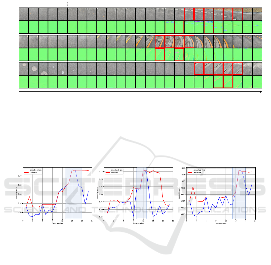
scene1

RGB

Normal

scene2

RGB

Normal

scene3

RGB

Normal

𝒕

first input 5 frames

1 2 3 4 5 6 7 8 9 10 11 12 13 14 15 16 17 18 19 20

Figure 8: These datasets, created by capturing and composing images through a camera, are presented for the evaluation of

anomaly detection in 3 different scenes. While only normal maps were utilized as inputs for the Long Short-Term Memory

(LSTM), RGB images are included for dataset illustration. Anomalous objects are deﬁned as follows: in Scene 1, while

stoppers; in Scene 2, a manhole and a curb of a sidewalk; in Scene 3, a curb of a sidewalk. The manhole that appears in the

ﬁrst input frames of scene 3 is embedded in the ground without any elevation difference. Therefore, they are excluded from

the detection targets in this experiment. In RGB images, frames enclosed in red represent anomaly frames in each scene, as

deﬁned in Section 4.2.1. In the normal maps generated using depth images, frames enclosed in red indicate frames that have

been identiﬁed as anomaly frames by the proposed method in each scene. These frames indicate instances where the distance

from the camera to anomalous objects is 2 meters or less. Each frame is resized to an image size of 192 × 256 pixels.

scene1 scene2 scene3

Figure 9: The graphs illustrate anomaly scores (Mean Squared Error loss between the feature vectors of the predicted normal

map at t + 1 and the normal map at t +1) obtained during anomaly detection for each scene of the dataset shown in Figure 8.

The blue curve represents the smoothed loss using the method described in (K. Hundman et al., 2018), while the red curve

represents the dynamically determined threshold. The region where anomaly frame numbers exist is represented by the blue

background.

the component perpendicular to the ground (y com-

ponent) are visualized using a jet color map. In other

words, the closer the value is to 0, the bluer the color

becomes, and the closer it is to 2, the darker the red

color becomes.

4.2.5 Discussion

Beginning the discussion on the results of Sec-

tion 4.2.2, Figure 9 reveals that in regions containing

anomaly frames, there is a discernible upward trend

in the loss. This trend signiﬁes an increase in the loss

between the feature vectors of the predicted normal

map at t + 1 and the normal map at t + 1. From the re-

sults in Table 1, it is evident that more than 30% of the

anomaly frames are detected in all scenes. Not identi-

fying every anomaly frame does not pose a signiﬁcant

practical concern. In this experiment, our objective

was to detect anomalies within a 2-meter range from

the handheld camera, capturing 4 frames per second.

Considering walking scenarios, moving 2 meters in

approximately 1 second is difﬁcult. Therefore, the

ability to detect some frames from the set of anomaly

frames within a few frames is deemed sufﬁcient to ef-

fectively avoid anomalies.

Next, the results of Section 4.2.3 is discussed. The

proposed method aims to detect anomalies by com-

paring the predicted normal map at t + 1 from the past

few frames with the normal map at t + 1. Therefore,

it is expected to detect changes in road conditions

and anomalies even on uneven road surfaces, such as

grassy areas. Observing Figure 10, it is evident that

VISAPP 2024 - 19th International Conference on Computer Vision Theory and Applications

252

first input 5 frames

1 2 3 4 5 6

7 8 9 10 11

12 13

14 15 16 17

18 19

𝒕

21 22 23 24 25 26 27

28 29 30 31

34 35 36 37

38 39

41 42 43 44 45

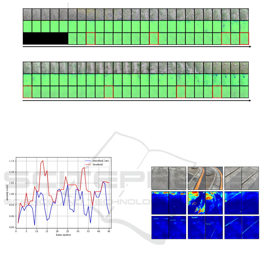
RGB

Reconstructed

normal map

Predicted

normal map

RGB

Reconstructed

normal map

Predicted

normal map

Figure 10: Dataset and anomaly detection results for verifying anomaly detection when road conditions change. The recon-

structed normal map is reconstructed using an encoder and decoder of the pre-trained Variational Autoencoder (VAE) from

the normal map derived from depth images captured by the camera. The predicted normal map is generated from the previous

5 frames of the reconstructed normal map. For instance, the ﬁrst frame of the predicted normal map is reconstructed from

the feature vector predicted by a Long Short-Term Memory (LSTM) from the feature vector of the ﬁrst input 5 frames of

the reconstructed normal map, using the decoder of the VAE. Frames enclosed in red boxes in the predicted normal map are

frames classiﬁed as anomaly frames. Each frame is resized to an image size of 192 × 256 pixels.

Figure 11: Graph depicting the variation in the threshold

and smoothed loss during anomaly detection using the pro-

posed method for the dataset in Figure 10.

anomalies are detected in frame 3, between frame 2

and 4, when the road conditions change. Additionally,

Frame 42 was detected as an anomaly frame when

a tree stump appears in the grassy area. Observing

Figure 11, it is evident that, even after entering the

grassy area around frame 3, the loss does not signif-

icantly increase. The anomaly score is kept below

1.05 until the appearance of a tree stump at frame 42.

This demonstrates the expected outcome that anoma-

lies can be detected based on the anomaly score be-

tween the predicted normal map at t +1 from the pre-

vious few frames of the road surface and the normal

map at t + 1, even when road surface conditions has

been changed.

scene1 scene2 scene3

frame11 frame12 frame10

frame12

frame16 frame17

RGB

Existing method

(K. Hundman

et al., 2018)

Proposed method

Figure 12: Examples of comparing the detection of anoma-

lous areas between the existing method (K. Hundman et al.,

2018) and the proposed method.

Regarding the results of the method (T. Voj

r and

J. Matas, 2023), examining Scene 1 in Figure 12 re-

veals that the method effectively detects anomalies

in the area of the car stopper, as evidenced by high

anomaly scores. However, when looking at Scenes

2 and 3, it becomes apparent that the method strug-

gles to detect anomalies in areas with curbs that have

colors similar to the road surface, as indicated by

the lower anomaly scores. In contrast, the proposed

method consistently detects anomalous regions in ar-

eas with anomalies when compared to non-anomalous

regions. This observation holds true for all cases in

Figure 12. This underscores the effectiveness of the

proposed method in anomaly detection within walk-

Anomaly Detection on Roads Using an LSTM and Normal Maps

253

ing scenarios, showcasing its ability to detect anoma-

lies without relying on color information.

The most likely reason for false detections is con-

sidered to be the inadequate performance of feature

extraction by the VAE. In this approach, anomaly de-

tection relies on the difference in feature vectors be-

tween that of the predicted normal map at t + 1 and

the normal map at t + 1. Hence, the performance of

the VAE’s encoder plays a crucial role in inﬂuencing

the outcomes. Enhancing the detection performance

is anticipated by achieving a more accurate feature ex-

traction for unknown normal maps using the VAE.

While there is still signiﬁcant room for improve-

ment in avoiding the misclassiﬁcation of normal (non-

abnormal) frames as anomaly frames in both Sec-

tion 4.2.2 and Section 4.2.3, the results presented

above effectively highlight the efﬁcacy of the pro-

posed method. This approach, utilizing normal maps

and anomaly detection, demonstrates its effectiveness

in detecting anomalies on the road.

5 CONCLUSION

In this paper, we propose a novel approach for detect-

ing road surface anomalies using normal maps and

anomaly detection. When walking, individuals may

unconsciously perceive that there is no danger based

solely on the color information of the road surface.

However, in reality, there could be anomalies that lead

to signiﬁcant accidents. Our method aims to address

the potential risks posed by these anomalies by pre-

dicting the normal map of the ground surface one is

about to walk on, leveraging a time series of normal

maps, and generating anomaly scores. The effective-

ness of our proposed method has been demonstrated

through experiments using the custom datasets. This

research, combining normal maps with anomaly de-

tection, contributes to advancements in the ﬁelds of

pedestrian assistance and anomaly detection.

REFERENCES

A. Kirillov, E. Mintun, N. Ravi, H. Mao, C. Rolland, L.

Gustafson, T. Xiao, S. Whitehead, A. C. Berg, W.

Lo, P. Dollar, and R. Girshick (2023). Segment any-

thing. In Proceedings of the IEEE/CVF International

Conference on Computer Vision (ICCV), pages 4015–

4026.

D. Ha and J. Schmidhuber (2018). World models. arXiv

preprint arXiv:1803.10122.

D. T. Shipmon, J. M. Gurevitch, P. M. Piselli, and S. T.

Edwards (2017). Time series anomaly detection; de-

tection of anomalous drops with limited features and

sparse examples in noisy highly periodic data. arXiv

preprint arXiv:1708.03665.

D.P. Kingma and J. Ba (2015). Adam: A method for

stochastic optimization. In International Conference

on Learning Representations (ICLR), pages 1–15.

Hunter, J. S. (1986). The exponentially weighted moving

average. Journal of quality technology, 18(4):203–

210.

I. Higgins, L. Matthey, A. Pal, C. Burgess, X. Glorot,

M. Botvinick, S. Mohamed, and A. Lerchner (2016).

beta-vae: Learning basic visual concepts with a con-

strained variational framework. In International Con-

ference on Learning Representations.

I. Vasiljevic, N. Kolkin, S. Zhang, R. Luo, H. Wang, F. Z.

Dai, A. F. Daniele, M. Mostajabi, S. Basart, M. R.

Walter, and G. Shakhnarovich (2019). Diode: A dense

indoor and outdoor depth dataset. arXiv preprint

arXiv:1908.00463.

J. Goh, S. Adepu, M. Tan, and Z. S. Lee (2017).

Anomaly detection in cyber-physical systems using

recurrent neural networks. In IEEE 18th International

Symposium on High Assurance Systems Engineering

(HASE), pages 140–145.

K. Hundman, V. Constantinou, C. Laporte, I. Colwell, and

T. Soderstrom (2018). Detecting spacecraft anomalies

using lstms and nonparametric dynamic thresholding.

In Proceedings of the 24th ACM SIGKDD Interna-

tional Conference on Knowledge Discovery & Data

Mining, pages 387–395.

K. Imai, I. Kitahara, and Y. Kameda (2017). Detecting

walkable plane areas by using rgb-d camera and ac-

celerometer for visually impaired people. In 3DTV

Conference: The True Vision-Capture, Transmission

and Display of 3D Video (3DTV-CON), pages 1–4.

K. Yanagihara, H. Takefuji, P. Sarakon, and H. Kawano

(2020). A method to detect steps on the sidewalks for

supporting visually impaired people in walking. In

Proceedings of the Fuzzy System Symposium (Japan

Society for Fuzzy Theory and Intelligent Informatics),

volume 36, pages 395–398.

L. Shen, Z. Li, and J. Kwok (2020). Time series anomaly

detection using temporal hierarchical one-class net-

work. In Advances in Neural Information Processing

Systems 33, pages 13016–13026.

N. Ding, H. Ma, H. Gao, Y. Ma, and G. Tan (2019).

Real-time anomaly detection based on long short-term

memory and gaussian mixture model. Computers &

Electrical Engineering, 79.

R.R. Selvaraju, M. Cogswell, A. Das, R. Vedantam, D.

Parikh, and D. Batra (2017). Grad-cam: Visual ex-

planations from deep networks via gradient-based lo-

calization. In IEEE International Conference on Com-

puter Vision, pages 618–626.

S. Hochreiter and J. Schmidhuber (2015). Anomaly detec-

tion in ecg time signals via deep long short-term mem-

ory networks. In 2015 IEEE International Conference

on Data Science and Advanced Analytics (DSAA),

pages 1–7.

T. Voj

r and J. Matas (2023). Image-consistent detection of

road anomalies as unpredictable patches. In Proceed-

VISAPP 2024 - 19th International Conference on Computer Vision Theory and Applications

254

ings of the IEEE/CVF Winter Conference on Applica-

tions of Computer Vision (WACV), pages 5491–5500.

W. Wu, L. He, W. Lin, Y. Su, Y. Cui, C. Maple, and S.

Jarvis (2020). Developing an unsupervised real-time

anomaly detection scheme for time series with multi-

seasonality. IEEE Transactions on Knowledge and

Data Engineering.

Y. Nonaka, H. Uchiyama, H. Saito, S. Yachida, and K.

Iwamoto (2023). Patch-based difference-in-level de-

tection with segmented ground mask. Electronics,

12(4).

Z. Z. Darban, G. I. Webb, S. Pan, C. C. Aggarwal,

and M. Salehi (2022). Deep learning for time se-

ries anomaly detection: A survey. arXiv preprint

arXiv:2211.05244.

Anomaly Detection on Roads Using an LSTM and Normal Maps

255