A Deep Analysis for Medical Emergency Missing Value Imputation

Md Faisal Kabir

and Sven Tomforde

Institute of Computer Science, Department of Intelligent Systems, University of Kiel,

Christian-Albrechts-Platz 4, Kiel, Germany

Keywords:

Medical Emergency System, Missing Value, Data Imputation, Autoencoder, Deep Learning.

Abstract:

The prevalence of missing data is a pervasive issue in the medical domain, necessitating the frequent deploy-

ment of various imputation techniques. Within the realm of emergency medical care, multiple challenges have

been addressed, and solutions have been explored. Notably, the development of an AI assistant for telenotary

service (TNA) encounters a signiﬁcantly higher frequency of missing values compared to other medical appli-

cations, with these values missing completely at random. In response to this, we compare several traditional

machine learning algorithms with denoising autoencoder and denoising LSTM autoencoder strategies for im-

puting numerical (continuous) missing values. Our study employs a genuine medical emergency dataset, which

is not publicly accessible. This dataset exhibits a signiﬁcant class imbalance and includes numerous outliers

representing rare occurrences. Our ﬁndings indicate that the denoising LSTM autoencoder outperforms the

conventional approach.

1 INTRODUCTION

Medical emergencies represent a paramount concern,

posing substantial challenges not only in addressing

patients’ life-threatening conditions but also in the

prompt assessment and treatment initiation faced by

healthcare professionals. This process is inherently

time-intensive. Therefore, an existing telenotary ser-

vice (TeleNotarzt, TNA) (Aachen, 2023) is being un-

dertaken to enhance support during medical emergen-

cies.

The successful categorization of diseases in future

emergency medical applications requires a substan-

tial dataset. Our dataset, sourced from a decade of

TNA operations in Aachen, Germany, includes mea-

surement data records for patients and their emer-

gency cases. However, numerous patient samples

lack essential parameters, potentially leading to inac-

curate classiﬁcation results. Furthermore, the dataset

displays a notable class imbalance and incorporates

outliers reﬂective of genuine medical events, which

are crucial for understanding speciﬁc diseases. This

study aims to investigate missing value imputation

techniques that effectively handle minority class in-

stances while accurately identifying outliers linked to

rare disease events.

https://orcid.org/0009-0000-2354-2193

https://orcid.org/0000-0002-5825-8915

Within this research paper, we propose two de-

noising autoencoder models, namely the conventional

denoising autoencoder and the denoising LSTM au-

toencoder, with the primary objective of addressing

missing value imputation. Subsequently, we per-

form a comparative analysis of both models with an

emphasis on optimization. Additionally, our pro-

posed model is systematically evaluated against var-

ious machine learning models and statistical tech-

niques, including mean imputations, K-nearest neigh-

bors (KNN), Iterative Imputer (I.Imp), Decision

Tree (D.Tree), and Linear Regression (LR). This is

the ﬁrst study to complete the missing imputation for

the emergency medical dataset, a corresponding real-

world-based. With this paper, we aim to answer the

question of which techniques are most suitable for

this kind of scenario and which challenges need to be

tackled.

The paper is organized as follows: Section 2 re-

views existing literature on missing data patterns,

techniques, and methodologies. Section 3 discusses

current state-of-the-art developments. Section 4 ex-

plains the formulation of proposed models, and Sec-

tion 5 details data description and preparation. Model

evaluation is covered in Section 6, while Section 7

analyzes experimental outcomes, presenting insights

and ﬁndings. Finally, Section 8 summarises the paper

and outlines future research directions.

Kabir, M. and Tomforde, S.

A Deep Analysis for Medical Emergency Missing Value Imputation.

DOI: 10.5220/0012457300003636

Paper published under CC license (CC BY-NC-ND 4.0)

In Proceedings of the 16th International Conference on Agents and Artiﬁcial Intelligence (ICAART 2024) - Volume 3, pages 1229-1236

ISBN: 978-989-758-680-4; ISSN: 2184-433X

1229

2 BACKGROUND

Missing values are a common problem in a dataset.

The causes of missing values are the data entry mech-

anism not working, updating the new system, human

error, system error, faulty measurements, etc. In this

case, the critical issue needs values for future product

improvement. So, it is necessary to know 1) types of

missing value, 2) strategies of missing value imputa-

tion and 3) imputation techniques.

2.1 Types of Missing Values

In situations where data are classiﬁed as Missing

Completely at Random (MCAR), there is an absence

of any discernible connection between missing and

non-missing values. In other words, missing and non-

missing variables contain no relationship. The miss-

ing value placed in a dataset is entirely random (Em-

manuel et al., 2021; Hameed and Ali, 2023). So, the

probability is represented as: P(X

, X

) = P(X

This equation indicates that the probability of miss-

ingness (X

) is not inﬂuenced by the observed data

) or the missing data (X

), as the conditional prob-

ability is equal to the unconditional probability (Em-

manuel et al., 2021; Hameed and Ali, 2023).

Missing at Random (MAR) considers if the miss-

ing data is connected to observed variables and has a

relationship between the subset of that variable. For

example, if we consider X

as an observed variable,

which is the person’s name, X

is age, X

is monthly

income, and other variables are different parameters.

Here X

is missing variables (Emmanuel et al., 2021;

Hameed and Ali, 2023). We can write that the proba-

bility of missing is P(X

, X

) = P(X

When the missing variable depends on itself and

the observed variable, we call it Missing Not at Ran-

dom (MNAR) (Emmanuel et al., 2021; Hameed and

Ali, 2023). This can be expressed as: P(X

, X

) =

f (X

2.2 Missing Data Handling

AI missing imputation divides into two parts: ma-

chine learning and deep learning. Deep learning is

a subsection of machine learning, but deep learning is

one of the best approaches to complete missing val-

ues. The Deep learning approach mainly focuses on

model-based and predicts missing values to achieve

the target dataset. Deep learning uses a neural net-

work with multiple layers to discover the dataset’s

complex pattern. Conversely, deep learning is com-

plicated to construct a model and requires high com-

putational capacity (Emmanuel et al., 2021; Liu et al.,

2023a; Sun et al., 2023; Liu et al., 2023b).

2.3 Missing Imputation Techniques

Machine learning missing value imputation tech-

niques based on Classiﬁcation and clustering mod-

els. Bayesian, neural network, decision tree, ran-

dom forest and support vector machine are con-

sidered classiﬁcation-based models. On the other

hand, k-means, subspace, self-organising map, and

kernel are clustering-based models. To complete

missing imputation, autoencoder (AE), variational

autoencoder (VAE), generative adversarial networks

(GANs), Long short-term memory (LSTM) networks,

and transformers are used in deep learning (Adhikari

et al., 2022; Emmanuel et al., 2021; Liu et al., 2023a;

Sun et al., 2023).

3 RELATED WORK

Recently, many methods have been employed for

missing data imputations across diverse data types

spanning various sectors. This section mainly con-

centrates on the application of these methods in the

context of medical and healthcare datasets. The cur-

rent state of the art reveals the utilization of multi-

ple models based on deep learning techniques for ad-

dressing missing data across various data types.

In the medical domain, missing imputation tech-

niques are extensively utilized for tabular static data,

signals, temporal data, images, and genetic and ge-

nomic data. Deep learning models have demonstrated

superior accuracy compared to alternative algorithms.

Typically, missing data imputation serves as a critical

step in data preprocessing, with the ultimate objec-

tive often being prediction or classiﬁcation analysis.

Concurrently, various statistical and machine learning

models are also employed to assess imputation accu-

racy for subsequent processes (Liu et al., 2023a).

Notably, multilayer perceptron (MLP) with gradi-

ent descent emerges as a successful method for imput-

ing missing values, showcasing superior performance

compared to other statistical methods such as mode,

random, hot-deck, KNN, decision tree, and random

forest (Pan et al., 2022). GapNet (Chang et al., 2022),

another approach rooted in the MLP model, exhibits

similar imputation performance as MLP with gradi-

ent descent. MLP models, known for their effective-

ness in handling static data, also demonstrate note-

worthy performance in genetic datasets, exempliﬁed

by deepMC (Mongia et al., 2020).

For temporal data, models such as Long Short-

Term Memory (LSTM), Recurrent Neural Network

ICAART 2024 - 16th International Conference on Agents and Artiﬁcial Intelligence

1230

(RNN), and Gated Recurrent Unit (GRU) are specif-

ically designed and proﬁcient in handling time se-

ries missing values. To predict hypertensive disor-

der in pregnancy (HDP) using pregnancy examination

data, a Bidirectional LSTM model outperforms cubic

spline interpolation, KNN ﬁlling, the LSTM model,

and the ST-MVL model (Lu et al., 2023). On the other

hand, a forward-to-backward bidirectional model em-

ploying missing imputation demonstrates enhanced

accuracy in predicting Alzheimer’s disease compared

to other methods (Ho et al., 2022).

Within the medical domain, autoencoders are ex-

tensively employed for missing value imputation. An

illustrative experiment utilized a sample autoencoder

to impute missing values using a dataset with ran-

domly masked values in the missing positions. This

approach was compared with mean imputation, re-

vealing superior results in favour of the autoencoder

method over mean imputation (Macias et al., 2021).

Additionally, employing a random mask as an auxil-

iary input proved beneﬁcial in assisting the network

to discern between missing and zero features. In

this context, autoencoders demonstrated superior per-

formance across ﬁve distinct datasets, namely Breast

Cancer Wisconsin (WDBC), Parkinson’s disease, di-

abetic data, Indian Liver Patient Dataset (ILPD),

and National Surgical Quality Improvement Program

(NSQIP). This performance surpassed that of the

support vector machine (SVM), k-nearest neighbour

(KNN), artiﬁcial neural network (ANN), linear re-

gression (LR), and random forest (RF) (Kabir and

Farrokhvar, 2022).

A stacked denoising autoencoder (DAE) was im-

plemented with a low-dimensional representation.

The weight matrix of the last layer in the encoder

was utilized as the transpose weight matrix in the ﬁrst

layer of the decoder (Abiri et al., 2019). In the Fram-

ingham Heart dataset, the process of missing impu-

tation was conducted using a DAE as the generator

within an Improved Generative Adversarial Network

(IGAN). Before inputting the data into the model,

missing values were ﬁlled using K-Nearest Neigh-

bors (KNN). Notably, IGAN demonstrated superior

performance when compared to Simple imputation,

KNN, MissForest, Neighborhood Aware Autoen-

coder (NAA), and Improved Neighborhood Aware

Autoencoder (INAA) (Psychogyios et al., 2022).

The current state of the art reveals numerous stud-

ies addressing missing imputation in various medical

datasets. However, no existing work has speciﬁcally

focused on addressing the challenge of emergency

medical missing data imputation. In response, we

study two autoencoder models—the Denoising Au-

toencoder and the Denoising LSTM Autoencoder for

the imputation of emergency medical data.

4 PROPOSED MISSING VALUE

IMPUTATION

4.1 Autoencoder

An autoencoder (AE) comprises an encoder and

a decoder. The encoder processes the input data

and generates an output that represents a reduced-

dimensional vector space, commonly referred to as

the latent space or information bottleneck. The math-

ematical functions governing the encoder and decoder

are denoted as f (x) = z and g(z) = x

′

. Let us pro-

vide a more detailed elaboration of these functions.

In the context of model construction for the encoder,

w1 and b1 represent the weight matrix and bias of the

ﬁrst layer, respectively. Here, x and f denote the in-

put and activation functions, leading to the presenta-

tion of the output as z. (Wang et al., 2016; Chen and

Guo, 2023) The equation can be expressed as follows:

z = f (w × x + b). Same as for the decoder, w

′

, b

′

and x

′

are weight, bias, activation function of decoder

output layer and reconstruction data presented. z is

the input of the decoder. So the equation presented

as: x

′

= g(w

′

× z + b

′

). Training an autoencoder loss

function is also an important issue. The loss func-

tion calculates how input data is reconstructed. To

deﬁne the loss function, the following expression is

used: L(x, g( f (x)))

4.2 Denoising Autoencoder

The denoising autoencoder (DAE) represents an ex-

tension of the standard autoencoder. While the AE is

designed to reconstruct input data, the DAE, in con-

trast, is tasked with reconstructing the original data

from noisy input. In essence, the encoder of the DAE

processes noisy data denoted as x

′′

, and the decoder

reconstructs the corresponding noise-free data, which

is presented as x. It is important to note that apart from

this distinction in their reconstruction objectives, both

the AE and DAE share an identical model construc-

tion. The input data of DAE adds some extra noise,

which could be random noise(Vincent et al., ; Vincent

et al., 2008).

Figure 1 illustrates our proposed DAE, delineat-

ing two distinct components: one for training the

DAE and the other one for imputation of missing val-

ues. Initially, the dataset was partitioned into two

sub-datasets: one is samples with missing values, and

the other contains samples with non-missing values.

A Deep Analysis for Medical Emergency Missing Value Imputation

1231

Figure 1: Denoising LSTM autoencoder imputation archi-

tecture.

The non-missing dataset adds some noise as mean

values in the ﬁrst block. The mean value replaces

the non-missing dataset’s exact location where data

are missing in the missing value dataset. So, the

encoder, decoder and the loss function of the DAE

model are expressed as follows: z = f (w × x

′′

+ b),

x = g(w

′

× z + b

′

) and L(x, g( f (x

′′

))).

The second block of Figure 1 depicts the impu-

tation procedure. In this process, complete the miss-

ing value with the mean value as noise in the missing

dataset. After training the model with the noisy com-

plete dataset. Now, test the missing values for imputa-

tion. The reconstruction data present imputation data.

We construct the model as simply as possible because

of the small dataset and reduce the overﬁtting.

4.3 LSTM Autoencoder

The denoising LSTM autoencoder is an extension of

DAE (Coto-Jimenez et al., 2018). Figure 1 depicts an

alternative DAE model, speciﬁcally built as a Denois-

ing Long Short-Term Memory Autoencoder (LSTM

DAE). It’s important to note that the primary dis-

tinction between the ﬁrst and second models lies in

the design of the encoder and decoder. The initial

DAE model employed conventional neurons for its

autoencoder, while the LSTM DAE model was con-

structed using LSTM components. Notwithstanding

this disparity, all other conﬁgurations and parameters

of the models remain consistent. Similarly, the second

block, corresponding to missing value imputations,

follows the same procedure. Another consideration

pertains to data preparation for LSTM; details on this

aspect are provided in the data preparation section.

5 DATA DESCRIPTION AND

PREPARATION

5.1 Dataset

In this research study, we harnessed emergency med-

ical data, which is not publicly accessible, and aimed

to address the challenge of missing value imputa-

tion. The data originated from emergency medical

cases involving numerous patients, thus constituting a

multifaceted dataset encompassing various attributes

and parameters, including categorical, numerical, and

text-based data. This dataset exhibited substantial

heterogeneity. Our focus primarily centred on numer-

ical data, such as blood pressure, oxygen levels, and

various measurements, which are inherently speciﬁc

to individual diseases. The dataset encompasses ap-

proximately 200 distinct diseases with varying preva-

lence. While some diseases are commonly encoun-

tered, others are quite rare, resulting in a pronounced

class imbalance within the dataset.

The dataset, comprising about 16,000 samples,

has an incidence of approximately 50% missing val-

ues. Of these samples, 9,834 are complete, and the

rest exhibit missing data. The missing values ap-

pear randomly, with little discernible interrelationship

among variables, suggesting a lack of inherent asso-

ciations. These omissions result from the data gen-

eration process, where telenotary doctors input in-

formation during emergency cases via telephone and

video calls without mandatory ﬁeld checks or re-

minder functions. A synthetic dataset mirroring the

actual distribution is available in the appendix.

5.2 Data Preparation

At ﬁrst, we separated the dataset into two parts: miss-

ing and non-missing datasets. To train a denoising

autoencoder, we need one noisy train dataset, which

will be reconstructed into original data. Traditionally,

extra noise in the training dataset and train the model.

We add the noise in a slightly different way, not using

random noise on the training dataset.

Figure 2 demonstrates the process of adding noise.

In this ﬁgure, there are two blocks presents. The ﬁrst

block shows a simple block diagram of how the pro-

cess is realized. The second block presents the same

as the ﬁrst block but in the form of a table representa-

tion of missing imputation. At ﬁrst, we have to iden-

tify the location of the missing values on missing sam-

ples. Then, we place the exact location on the com-

plete dataset and replace the mean of the non-missing

dataset. Now, this non-missing dataset gets corrupted

or noisy(Ma et al., 2020).

We employed various missing data percentages

for imputation within the dataset. These missing data

percentages encompassed values of 20%, 30%, 40%,

and 50%.

ICAART 2024 - 16th International Conference on Agents and Artiﬁcial Intelligence

1232

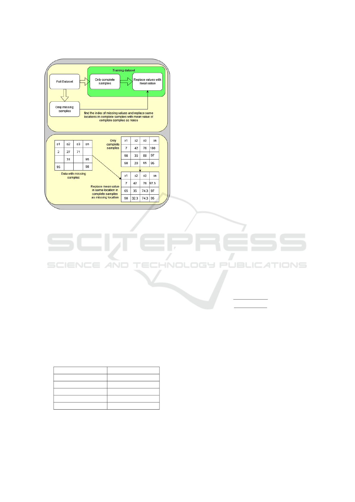
Figure 2: Data preparation for denoising autoencoder.

6 EXPERIMENTS

This experiment section describes two model conﬁgu-

rations: the activation function, the evaluation matrix

and the results.

6.1 Model Conﬁguration

From the complete dataset with no missing values,

12% was assigned for creating the ground truth, and

the rest constituted the training dataset. Within the

training dataset, 70% was used for training, and the

remaining 30% served for validation. To optimize re-

sults, we adopted a trial-and-error approach, leading

to a variable training epoch. Given the highly class

imbalance and presence of outliers, we implemented

early stopping to address potential overﬁtting.

Table 1: Model hyperparameter and hyperparameter range.

Parameter value range

Learning rate 0.0001 ≤ n ≤ 0.01

Batch size 16 ≤ n ≤ 64

Hidden layers 0 ≤ n ≤ 2

Hidden layers units 16 ≤ n ≤ 64

Activation function Relu and Softmax

Table 1 outlines the hyperparameters and their

corresponding ranges utilized in both models, care-

fully selected based on superior performance com-

pared to alternative conﬁgurations. Key hyperparam-

eters inﬂuencing model construction include hidden

layers, units within hidden layers, activation func-

tions, learning rate, and batch size. Learning rates

spanned from 0.0001 to 0.01, with batch sizes rang-

ing from 16 to 64. An extended exploration con-

sidered learning rates from 0.00001 to 0.1 and batch

sizes from 4 to 512, with larger batch sizes incorpo-

rating batch size normalization layers. Hidden layer

parameters were optimized through exploration, vary-

ing from 0 to 2 layers and an additional experiment

ranging from 0 to 5 layers. Hidden layer units ranged

from 16 to 64, with an extensive analysis consider-

ing units from 4 to 512. The Relu activation function

was predominantly used in hidden layers, while soft-

max was exclusively employed in the dense output

layer. Various activation functions were evaluated for

their efﬁcacy in hidden layer presentations. The mean

squared error (MSE) loss function served as the train-

ing metric, assessing loss across both training and val-

idation datasets. This paper introduces two models

with 24 distinct hyperparameter combinations for in-

dividual missing percentages, each trained separately.

The identiﬁed hyperparameter ranges are crucial for

model training and missing imputation.

6.2 Evaluation Matrix

In the test experiment, several evaluation matrices

were performed to test the ground truth and recon-

struction of ground truth. Other measures have also

been analysed, but the RSME provides the most re-

liable scores. This paper includes only root mean

square error (RMSE). The RMSE is deﬁned as

∑

i=1

( ˆy

− y

)

In the equation above, n refers to the number of

observations. ˆy

and y

are presents as predicted and

original data respectively (Tyagi et al., 2022).

6.3 Results

In this section, we analyze the experiment outcomes,

emphasizing the optimal performance achieved with

diverse hyperparameters. Table 2 exclusively show-

cases the top result among 24 unique model conﬁgu-

rations. For each missing percentage category (e.g.,

20%, 30%, etc.), the best-performing model is high-

lighted from the 24 conﬁgurations.

Overall, eight results were displayed from 96

models. So, we present only two ﬁgures for ground

truth and predicted ground truth. We choose for 30%

missing imputation results and comparison.

A Deep Analysis for Medical Emergency Missing Value Imputation

1233

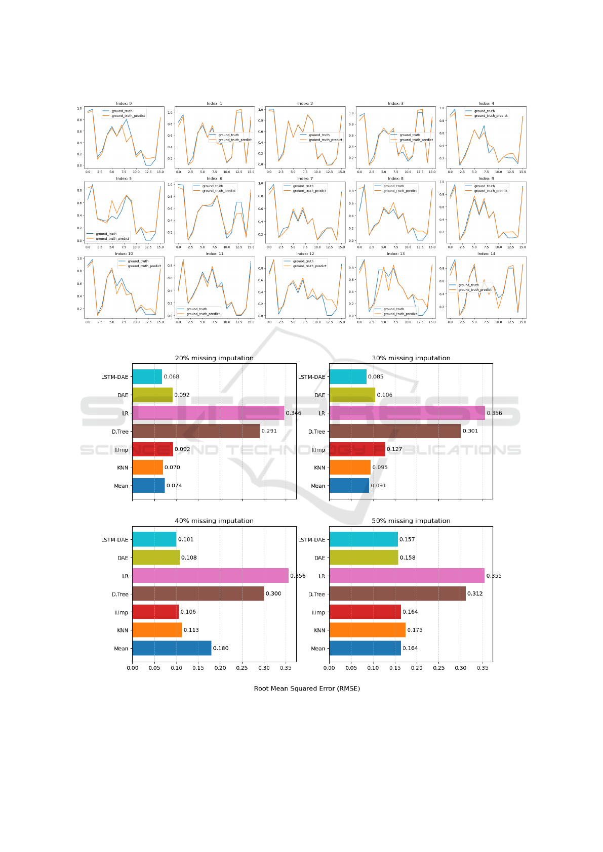
Figure 3: Comparision of ground truth and predicted ground truth for LSTM DAE.

Figure 4: Comparision of seven different missing imputation methods.

ICAART 2024 - 16th International Conference on Agents and Artiﬁcial Intelligence

1234

Table 2: LSTM DAE model compared with several ma-

chine learning and statistical methods for missing imputa-

tion. Here is the RMSE value, which is compared to the

ground truth generated.

model

\missing

20% 30% 40% 50%

Mean 0.07369 0.09149 0.18007 0.16381

KNN 0.06960 0.09472 0.11314 0.17491

I.Imp 0.09231 0.12739 0.10607 0.14498

D.Tree 0.29109 0.30084 0.30034 0.31181

LR 0.34629 0.35624 0.35604 0.35461

DAE 0.09180 0.10596 0.10763 0.15755

LSTM

DAE

0.06792 0.08523 0.10083 0.15702

Figure 3 illustrates the comparison between the

actual ground truth and the predicted values based on

the ground truth. The ﬁgure comprises 15 subplots,

with each subplot representing distinct features. In

Figure 3, the original ground truth is depicted by blue

lines, while the orange lines indicate the predicted

values.

7 DISCUSSION

The results section presents the outcomes of the miss-

ing values imputation across various missing per-

centage scenarios, ranging from 20% to 50% miss-

ing. Notably, the LSTM DAE consistently outper-

forms the standard DAE in every missing data case.

The proposed models perfectly capture the class-

imbalanced data.

The optimal DAE model for 20% missing imputa-

tion features a single hidden layer with 64 units for

both the encoder and decoder, outperforming other

conﬁgurations with a learning rate of 0.0001 and a

batch size of 64. Similarly, for 30%, 40%, and 50%

missing imputation, the DAE model performs best

with the same conﬁguration, adjusting the learning

rate slightly to 0.001. A lower learning rate enhances

model accuracy as the missing imputation increases.

For the LSTM DAE, the rise in missing values cor-

responds to a reduction in the number of hidden layer

units. Conversely, an increase in learning rate and

batch size improves performance as missing values

decrease. Speciﬁcally, conﬁgurations with 64 units

for the hidden layer, a learning rate of 0.0001, and

a batch size of 16 exhibit superior performance for

20%, 30%, and 40% missing values compared to all

other setups. Conversely, the model for 50% missing

values imputation outperforms when conﬁgured with

32 hidden layer units, a learning rate of 0.001, and a

batch size of 32.

Both models demonstrate their peak performance

when the proportion of missing values remains below

30%; beyond this threshold, their efﬁcacy declines.

Importantly, LSTMs, typically applied to time series

data, prove effective for numerical data even without

a temporal dimension, surpassing the performance of

traditional DAE models in such scenarios.

Moreover, we conducted a comparative analysis

of several machine-learning models, which are shown

in Figure 4. Both Mean imputation and KNN demon-

strate a performance proximity to LSTM-DAE when

tasked with imputing 20% and 50% missing values.

Conversely, DAE yields results comparable to the It-

erative Imputer (I.Imp) technique. For the imputa-

tion of 30% missing values, Mean and KNN tech-

niques exhibit similar performance to LSTM-DAE,

with KNN demonstrating a decrease in accuracy as

missing values escalate. Throughout all scenarios,

Decision Tree (D.Tree) and Linear Regression (LR)

consistently exhibit lower performance relative to the

other techniques. Furthermore, LSTM-DAE consis-

tently outperforms all other models in all instances of

missing data.

In this experiment, we identiﬁed limitations in

both data preprocessing and the employed models.

In the data preprocessing stage, mean values were

introduced as noise at the locations of missing val-

ues within the complete dataset. However, this ap-

proach may have limitations when the missing dataset

is larger than the non-missing dataset. It proves effec-

tive only when the missing value dataset is consis-

tently smaller than the non-missing dataset.

8 CONCLUSIONS

Imputing missing data in emergency medical datasets

presents a signiﬁcant challenge, especially when deal-

ing with class imbalance and outliers, where missing

values occur randomly. To tackle this, we utilized

two models: the denoising autoencoder and the de-

noising LSTM autoencoder. Optimal hyperparameter

tuning is essential to effectively address class imbal-

ance during imputation. We compare our proposed

models with various machine learning models, and

our results demonstrate that the denoising LSTM au-

toencoder surpasses all other models in this context.

Future investigations will explore additional deep-

learning models, such as variational autoencoder,

generative adversarial network, and transformer, for

imputing missing values in both categorical and

continuous numerical data. The resulting imputed

datasets will be utilized in multi-label classiﬁcation

tasks to assess the effectiveness of various imputation

A Deep Analysis for Medical Emergency Missing Value Imputation

1235

techniques, with classiﬁcation performance serving as

the evaluation metric.

ACKNOWLEDGEMENTS

This work was funded by the German Ministry of

Education and Research (Bundesministerium f

ur Bil-

dung und Forschung) as part of the project “KI-

unterst

utzter Telenotarzt (KIT2)” under grant number

13N16402. We would like to thank them for their sup-

port.

REFERENCES

Aachen, U. (2023). https://www.telenotarzt.de/. Teleno-

tarzt.

Abiri, N., Linse, B., Ed

en, P., and Ohlsson, M. (2019). Es-

tablishing strong imputation performance of a denois-

ing autoencoder in a wide range of missing data prob-

lems. Neurocomputing, 365:137–146.

Adhikari, D., Jiang, W., Zhan, J., He, Z., Rawat, D. B.,

Aickelin, U., and Khorshidi, H. A. (2022). A Com-

prehensive Survey on Imputation of Missing Data

in Internet of Things. ACM Computing Surveys,

55(7):133:1–133:38.

Chang, Y.-W., Natali, L., Jamialahmadi, O., Romeo, S.,

Pereira, J. B., Volpe, G., and Initiative, f. t. A. D. N.

(2022). Neural network training with highly incom-

plete medical datasets. Machine Learning: Science

and Technology, 3(3):035001. Publisher: IOP Pub-

lishing.

Chen, S. and Guo, W. (2023). Auto-encoders in deep learn-

ing—a review with new perspectives. Mathe-

matics, 11(8).

Coto-Jimenez, M., Goddard-Close, J., Di Persia, L.,

and Leonardo Ruﬁner, H. (2018). Hybrid Speech

Enhancement with Wiener ﬁlters and Deep LSTM

Denoising Autoencoders. In 2018 IEEE Interna-

tional Work Conference on Bioinspired Intelligence

(IWOBI), pages 1–8.

Emmanuel, T., Maupong, T., Mpoeleng, D., Semong, T.,

Mphago, B., and Tabona, O. (2021). A survey on

missing data in machine learning. Journal of Big

Data, 8(1):140.

Hameed, W. M. and Ali, N. A. (2023). Missing value im-

putation techniques: A survey. UHD J. Sci. Technol.,

7(1):72–81.

Ho, N.-H., Yang, H.-J., Kim, J., Dao, D.-P., Park, H.-R., and

Pant, S. (2022). Predicting progression of Alzheimer’s

disease using forward-to-backward bi-directional net-

work with integrative imputation. Neural Networks,

150:422–439.

Kabir, S. and Farrokhvar, L. (2022). Non-linear missing

data imputation for healthcare data via index-aware

autoencoders. Health Care Management Science,

25(3):484–497.

Liu, M., Li, S., Yuan, H., Ong, M. E. H., Ning, Y., Xie,

F., Saffari, S. E., Shang, Y., Volovici, V., Chakraborty,

B., and Liu, N. (2023a). Handling missing values in

healthcare data: A systematic review of deep learning-

based imputation techniques. Artiﬁcial Intelligence in

Medicine, 142:102587.

Liu, M., Li, S., Yuan, H., Ong, M. E. H., Ning, Y., Xie,

F., Saffari, S. E., Shang, Y., Volovici, V., Chakraborty,

B., and Liu, N. (2023b). Handling missing values in

healthcare data: A systematic review of deep learning-

based imputation techniques. Artiﬁcial Intelligence in

Medicine, 142:102587.

Lu, X., Yuan, L., Li, R., Xing, Z., Yao, N., and Yu,

Y. (2023). An Improved Bi-LSTM-Based Missing

Value Imputation Approach for Pregnancy Examina-

tion Data. Algorithms, 16(1):12. Number: 1 Pub-

lisher: Multidisciplinary Digital Publishing Institute.

Ma, Q., Lee, W.-C., Fu, T.-Y., Gu, Y., and Yu, G. (2020).

MIDIA: exploring denoising autoencoders for missing

data imputation. Data Mining and Knowledge Discov-

ery, 34(6):1859–1897.

Macias, E., Serrano, J., Vicario, J. L., and Morell, A.

(2021). Novel Imputation Method Using Average

Code from Autoencoders in Clinical Data. In 2020

28th European Signal Processing Conference (EU-

SIPCO), pages 1576–1579. ISSN: 2076-1465.

Mongia, A., Sengupta, D., and Majumdar, A. (2020).

deepMc: Deep Matrix Completion for Imputation of

Single-Cell RNA-seq Data. Journal of Computational

Biology, 27(7):1011–1019. Publisher: Mary Ann

Liebert, Inc., publishers.

Pan, H., Ye, Z., He, Q., Yan, C., Yuan, J., Lai, X., Su, J.,

and Li, R. (2022). Discrete Missing Data Imputation

Using Multilayer Perceptron and Momentum Gradi-

ent Descent. Sensors, 22(15):5645. Number: 15 Pub-

lisher: Multidisciplinary Digital Publishing Institute.

Psychogyios, K., Ilias, L., and Askounis, D. (2022). Com-

parison of Missing Data Imputation Methods us-

ing the Framingham Heart study dataset. In 2022

IEEE-EMBS International Conference on Biomed-

ical and Health Informatics (BHI), pages 1–5.

arXiv:2210.03154 [cs].

Sun, Y., Li, J., Xu, Y., Zhang, T., and Wang, X. (2023).

Deep learning versus conventional methods for miss-

ing data imputation: A review and comparative study.

Expert Systems with Applications, 227:120201.

Tyagi, K., Rane, C., Harshvardhan, and Manry, M. (2022).

Regression analysis. In Artiﬁcial Intelligence and Ma-

chine Learning for EDGE Computing, pages 53–63.

Elsevier.

Vincent, P., Larochelle, H., Bengio, Y., and Manzagol, P.-

A. (2008). Extracting and composing robust features

with denoising autoencoders. In Proceedings of the

25th international conference on Machine learning -

ICML ’08, pages 1096–1103, Helsinki, Finland. ACM

Press.

Vincent, P., Larochelle, H., Lajoie, I., Bengio, Y., and Man-

zagol, P.-A. Stacked Denoising Autoencoders: Learn-

ing Useful Representations in a Deep Network with a

Local Denoising Criterion.

Wang, Y., Yao, H., and Zhao, S. (2016). Auto-encoder

based dimensionality reduction. Neurocomputing,

184:232–242.

ICAART 2024 - 16th International Conference on Agents and Artiﬁcial Intelligence

1236