Directional Filter for Tree Ring Detection

emi Decelle

, Phuc Ngo

, Isabelle Debled-Rennesson

, Fr

eric Mothe

and Fleur Longuetaud

Univ. Lyon, Univ. Lyon 2, CNRS, INSA Lyon, UCBL, LIRIS, UMR5205, France

Universit

e de Lorraine, CNRS, LORIA, UMR 7503, Vandoeuvre-l

es-Nancy, F-54506, France

Universit

e de Lorraine, AgroParisTech, INRAE, SILVA, F-54000 Nancy, France

Keywords:

Polar Quad-Tree Decomposition, Conﬁdence Map, Tree Ring Width Estimation, Cross-Section Wood Image.

Abstract:

This paper presents an approach to automatically detect tree rings and subsequent measurement of annual ring

widths in untreated cross-section images. This approach aims to offer additional insights on wood quality. It is

composed of two parts. The ﬁrst one is to detect tree rings by using directional ﬁlters together with an adaptive

reﬁning process allowing to extract the rings from radial information for different angles around the tree pith.

The second step consists in building a conﬁdence map by considering polar quad-tree decomposition which en-

ables us to identify the relevant regions of image for conducting the tree ring width measurements.The method

is evaluated on two public datasets, demonstrating good performance in both detection and measurement. The

source code is available at https://gitlab.com/Ryukhaan/treetrace/-/tree/master/treerings.

1 INTRODUCTION

Measuring tree rings of wood cross-sections is widely

used to study tree growth. By measuring and dating

all the tree rings from the center of the tree (pith) to-

ward the bark, it is possible to reconstruct the past life

of the tree and make assumptions about its growth

conditions, including climate. Tree-rings are tradi-

tionally hand-measured, a process that demands sig-

niﬁcant time and human effort. In the past, several

studies have been proposed for automating the detec-

tion of tree rings using computer vision techniques

(e.g., (Conner et al., 1998; Laggoune et al., 2005)).

However, these methods work on well-prepared wood

samples and function in a semi-automatic manner.

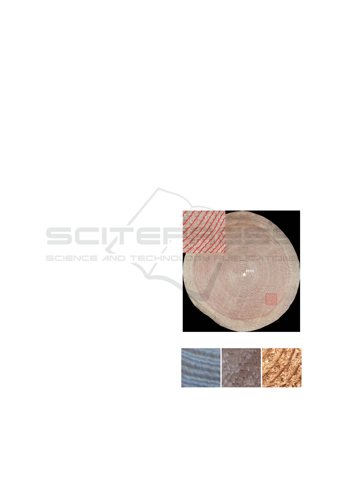
In this work, we are interested in automatic tree

ring analysis on color images of rough and untreated

log ends (see Figure 1). Such images may exhibit dis-

turbances like blurring, sawing marks or ambient light

variations, which make the analysis more challenging

(see wood patches in Figure 2). Furthermore, tree ring

detection remains an active research topic today be-

cause of the difﬁculty of detection on certain species,

particularly hardwoods (e.g., oak, beech, alder).

Recent studies in this area are often based on deep

learning approaches (e.g., (Fabija

nska and Danek,

2018; Marichal et al., 2023b; Pol

cek et al., 2023)).

Most of these methods work with radial cores or strips

of wood which provide partial information about the

tree-ring structure. Nevertheless, growth rings can

also be measured on a more macro scale, utilizing en-

Figure 1: Rough wood cross-section RGB image.

Figure 2: Exhibit disturbances of wood cross-section.

tire wood cross-section images, with the aim of pro-

viding information about the wood’s quality. For soft-

852

Decelle, R., Ngo, P., Debled-Rennesson, I., Mothe, F. and Longuetaud, F.

Directional Filter for Tree Ring Detection.

DOI: 10.5220/0012457000003654

Paper published under CC license (CC BY-NC-ND 4.0)

In Proceedings of the 13th International Conference on Pattern Recognition Applications and Methods (ICPRAM 2024), pages 852-859

ISBN: 978-989-758-684-2; ISSN: 2184-4313

woods (e.g., Douglas ﬁr, pine, spruce), narrow rings

are generally associated with a good mechanical qual-

ity for use in construction and therefore also have an

inﬂuence on the price of wood.

This article addresses the automatic measurement

of growth rings, for use in forests or sawmills, to en-

able better quality assessment of logs. This work de-

scribes a method to automatically detect tree rings on

segmented untreated log images by taking advantage

of general structure of tree cross-sections. More pre-

cisely, the method utilizes directional ﬁlters together

with an adaptive reﬁning process to extract tree rings

from radial information for different angles around

the pith. From the detected tree rings, we generate

a conﬁdence map by considering polar quad-tree de-

composition of the input image. This map enables us

to identify the most relevant regions of image for con-

ducting measurements, such as tree ring widths. The

method is evaluated on two public datasets (Longue-

taud et al., 2022; Marichal et al., 2023b) containing

untreated cross-sectioned wood images. Comparisons

are made with recent deep-learning approaches (Chen

et al., 2018) to demonstrate its good performance in

both detection and measurement. The source code is

available at https://gitlab.com/Ryukhaan/treetrace/-/

tree/master/treerings.

2 RELATED WORKS

In this section, we summarize existing algorithms ap-

plied on comparable unprepared images, resembling

those examined in this paper. In particular, our focus

is primarily on recent algorithms that might be partic-

ularly relevant to our speciﬁc case. More details of

various methods for tree ring detection can be found

in (Marichal et al., 2023b, Section 2).

(Fabija

nska and Danek, 2018) proposed an auto-

matic tree-ring boundary detector built upon the U-

Net convolutional network. The proposed method

focuses on wood core samples of tree ring porous

species. They achieved a precision of 97% and a re-

call of 96%. It is mentioned that the tree-ring bound-

aries are accurately aligned with the real ones. How-

ever, minimal manual adjustments are needed, pri-

marily around the pith, where tree-ring boundaries are

less distinct, displaying varying tilts and orientations.

Besides, they exclusively utilized core wood images

rather than full cross-sections of tree log ends.

(Makela et al., 2020) proposed automated meth-

ods for locating the pith (center) of a tree disk, and

ring boundaries. The proposed methods are based on

combination of standard image processing techniques

and tools from topological data analysis. However,

these methods were assessed using 2D slices from 3D

X-ray CT images of cross-sectioned tree trunks. Nei-

ther the code nor the data are publicly available.

(Gillert et al., 2023) addressed the problem of de-

tecting tree rings on whole cross-section images as an

instance segmentation task. For that, they proposed

an iterative method, called Iterative Next Boundary

Detection (INBD). More precisely, an input image is

passed through a semantic segmentation network that

detects 3 classes: background, ring boundaries and

ring center. Then, a polar grid is sampled starting

from the detected ring center and passed to the INBD

network to detect the next ring. The latter is repeated

until the background is encountered. Their method

was exclusively applied to microscopy images.

(Pol

cek et al., 2023) presented a supervised Mask

R-CNN for detection and measurement of tree-rings

from coniferous species. The CNN was trained and

validated on RGB images of cross-dated microtome-

cut conifers, with over 8000 manually annotated

rings. Different pre- and post-processing have been

applied to improve the model accuracy. They ob-

tained a precision of 94.8% and a recall of 98.7%

compared to cross-validated human detection. How-

ever, as most of the reviewed results, the approach

works on cores rather than the whole cross-section.

(Marichal et al., 2023b) introduced a novel non-

deep-learning approach to describe rings. A ring is

composed of nodes linked between them which create

a chain. A node is always on ray outwards from the

pith. A chain is a ring if it is closed. All rings form

a set called a spider web. Their deﬁnition allows to

ﬁt better tree rings. Their approach focuses on creat-

ing the spider web which is the closest to the rings on

the cross-section image. Their results show a F-score

of 89% on the UruDendro dataset (Marichal et al.,

2023a). However, the cross-section were smoothed

with a handheld planer and a rotary sander, meaning

that the cross-section is not raw. Their code is pub-

licly available.

3 METHOD

Our tree-ring detection (TRD) algorithm is based on

directional approach. Indeed, rings are roughly con-

centric, even if their shape is irregular (mainly at the

border of the log). This leads to the following charac-

teristics:

• Two rings will never overlap;

• A ray traced outwards from the pith will cross

each ring only once;

• A ring is delimited by two edges.

Directional Filter for Tree Ring Detection

853

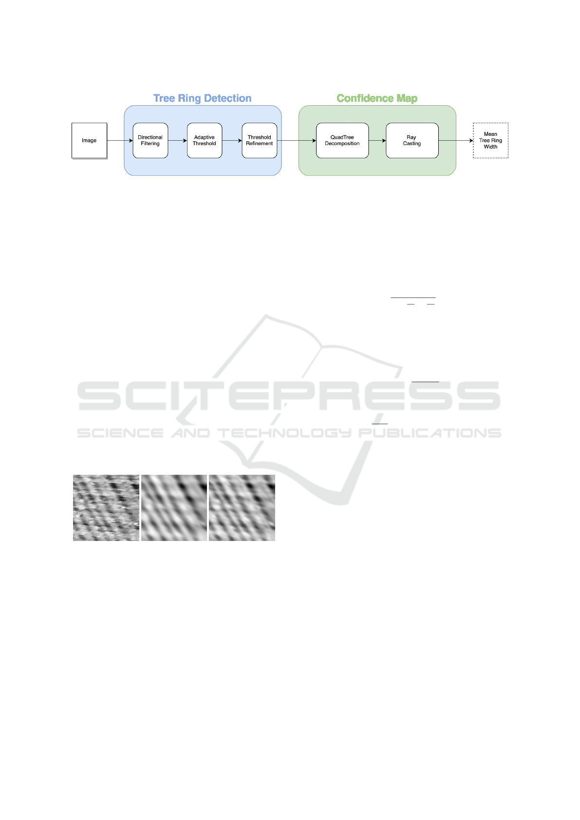
Figure 3: The global overview of our method.

Our method is compose of two parts. The ﬁrst

one focuses on TRD. The second one will estimate re-

gions where the detection should be good enough to

process some measurements, e.g., mean of tree ring

widths. The big picture of our method is shown in

Figure 3. The key feature of our proposal is that TRD

and estimation are separated, allowing to easily re-

place either step in future works.

3.1 Tree Ring Detection (TRD)

In order to delineate tree rings, we assume that the log

end image is segmented (Decelle et al., 2023; Wim-

mer et al., 2021). First, the input RGB image is con-

verted into grayscale using usual formulae.

The next step aims at highlighting tree ring transi-

tions and reducing noisy using directional ﬁlters. For

this, we assume that the pith position is known. Au-

tomatic algorithms have already been proposed for

this task (Norell and Borgefors, 2008; Kurdthongmee,

2020; Decelle et al., 2022).

3.1.1 Directional Filtering

(a) Input image (b) Lorentz (c) Gaussian

Figure 4: One example to highlight the choice of Lorentz

function instead of Gaussian function in Equation 2. Tree

rings are more connected with the Lorentz function than

gaussian function.

At ﬁrst, we need a ﬁlter that preserve edges of the

input image I, i.e. it preserves the ring boundaries.

In order to reduce noise along the tangential direc-

tion of tree rings, we consider a modiﬁed directional

Gaussian ﬁlter. The standard Gaussian domain ker-

nel exhibits symmetry relative to the window center.

To address the smoothing of image structures while

incorporating orientation and anisotropy, we use an

oriented kernel inspired by (Venkatesh and Seelaman-

tula, 2015). Let p = (p

, p

) ∈ I be the pixel to update

and q = (q

, q

) ∈ V (p) be pixels in its neighborhood.

In practice, V (p) is a window of size n ×n pixels.

′

(p) =

∑

q∈V (p)

f (p − q)I (q

− p

, q

− p

) (1)

where

f =

1 +

(2)

with

= (q

− p

)cos(θ)−(q

− p

)sin(θ)

= (q

− p

)sin(θ)+(q

− p

)cos(θ)

and θ is the angle between p and the pith c.

θ = arctan (

− c

) (3)

The parameters σ

and σ

control the kernel width

in x-axis and y-axis, respectively. We used the

Lorentz function

1+x

over a Gaussian function be-

cause the former one is more spread in the direction

θ than the latter one. This allows to ﬁlter more in

the direction of θ than using a Gaussian. Figure 4

shows the difference between the Lorentz and Gaus-

sian function with same pamareters for both. We can

observe that tree rings show better connection charac-

teristics with Lorentz than with a Gaussian function.

Figure 5 shows an example of the result obtained with

the proposed directional ﬁlter.

This ﬁlter is also interesting for its computational

efﬁciency. Since the kernel has to be computed

for each pixel, having a fast kernel computation is

needed. Moreover, reducing time for ﬁltering will al-

lows us to spend more time in selection area for mea-

suring tree ring widths (see Section 3.2).

3.1.2 Adaptive Threshold

After the ﬁltering, we need to ﬁnd the tree ring bound-

ary. This is done by two steps: the ﬁltered image is

ﬁrst thresholded, then the result is reﬁned. We pro-

pose to use a fast threshold: adaptive mean threshold

(Gonzalez, 2009). The threshold value is the mean of

the neighbourhood intensity minus a constant C. An

example is given in Figure 6 (left).

ICPRAM 2024 - 13th International Conference on Pattern Recognition Applications and Methods

854

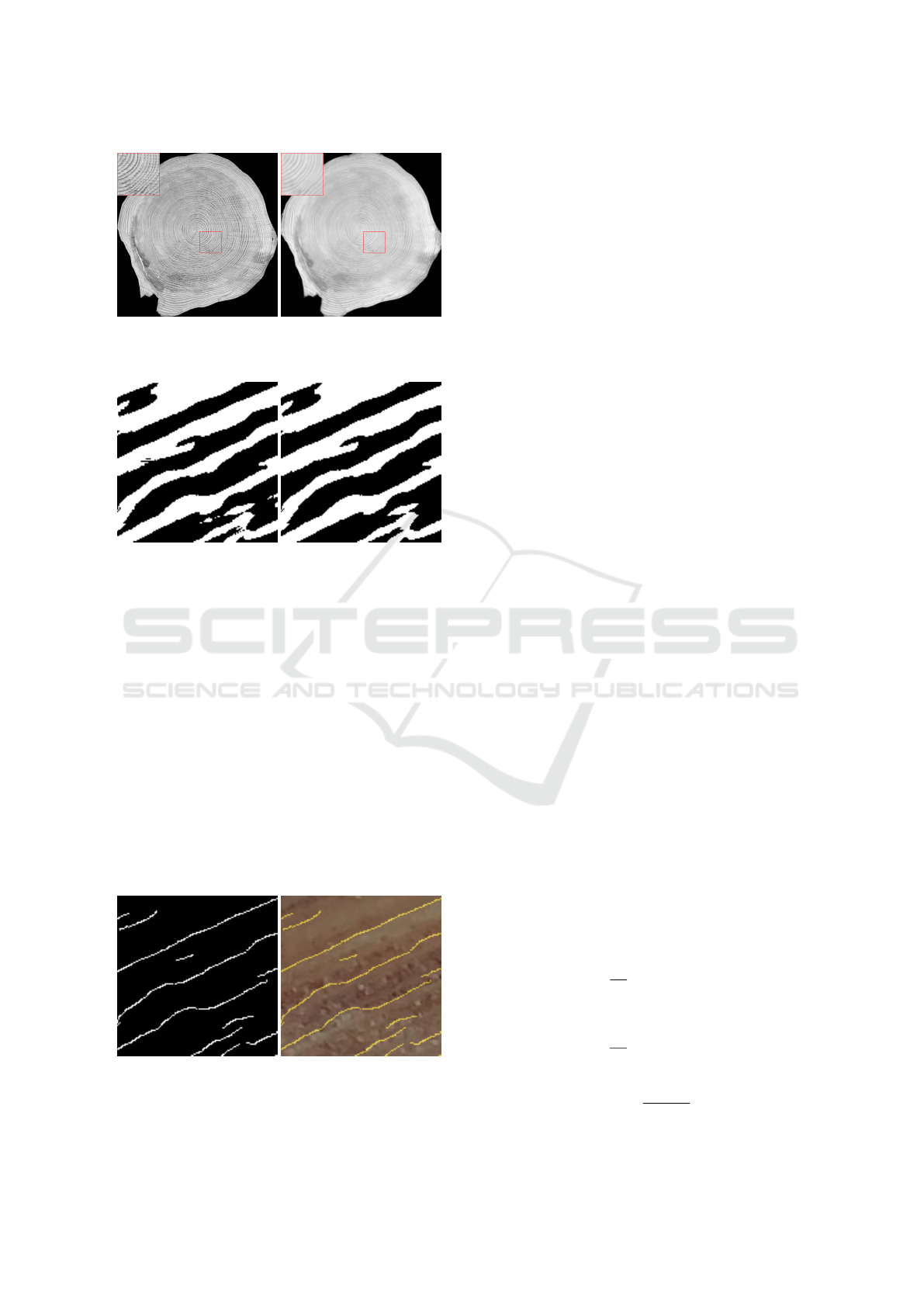
Figure 5: Left: Grayscale image. Right: Filtered image. At

the top left of the images, a zoom of the red rectangle.

Figure 6: Left: Raw thresholded image. Right: Thresholded

image after removing small areas.

3.1.3 Thinning

The previous adaptive threshold leads to thick tree

rings. In order to make them thinner, we suggest the

following steps. We remove all small connected com-

ponents. Since such components have not enough in-

formation to estimate tree rings widths. For that, we

ﬁrst apply dilatation morphology in order to reconnect

the regions. Then, if a region has less than 200 pixels,

it is removed. This is illustrated in Figure 6 (right).

Finally, we focus on transitions from latewood

(low intensity) to earlywood (high intensity) from the

pith outwards (i.e. from the pith to the bark). It corre-

sponds to a transition between white and black pixels

according to the outward direction from the pith. A

result of the thinning process is given in Figure 7.

Figure 7: Left: Result obtained after thinning the previous

thresholded image. Right: Delineation over the raw RGB

image.

3.2 Conﬁdence Map (CM)

Instead of trying to fully reconnect the detected seg-

ments to form closed rings, we propose here to parti-

tion the images into regions. We aim to identify the

most relevant regions to make measurements. For that

we will attribute a conﬁdence value to each region,

which will be seen as a conﬁdence map (CM).

3.2.1 Polar Quad-Tree Decomposition

Since tree rings are close to concentric circles, we de-

cide to split the image according to a polar quad-tree

decomposition. Such a decomposition is well-known

to decompose an image into regions in a recursive

way. This technique reveals information about the im-

age structure, and in our case, the information about

how well tree rings have been segmented.

The pith is the center of the decomposition. The

ﬁrst (and biggest) region is a circle with the pith as

center and a radius covering the cross-section. There

are three conditions to stop the subdivision process:

1. the region should be not too large to estimate

some directional characteristics. So, we suggest

to split until the tree depth reaches ρ

min

;

2. the region should be not too small in order to have

signiﬁcant measurements. This purpose is done

by stop splitting if the depth is greater than ρ

max

;

3. ﬁnally, the orientations in each region are all ho-

mogeneous.

Indeed, even if the detected tree rings are not glob-

ally connected, at a local level they are. Then, the

orientations should be homogeneous in such region.

This is why we choose the third criterion to stop or

continue the subdividing.

To estimate local orientations, we use discrete ge-

ometry. More precisely, the tool proposed in (Decelle

et al., 2021). However, this method is a little bit time-

consuming. Therefore, we decide to apply it for d

random selected points in each region. Each point

provides us a set of orientations.

At the end, we obtain N

possible orientations θ

The homogeneous criterion is the variance of those

orientations. Set:

S =

i=N

∑

i=1

sin(2θ

)

and

C =

i=N

∑

i=1

cos(2θ

)

The variance is computed as follows:

R =

Directional Filter for Tree Ring Detection

855

Figure 8: Example of polar quad-tree decomposition. We

show non-thin segmentation to hightlight link between seg-

mentation and evaluated conﬁdence.

By deﬁnition, R is in range of 0 and 1. This al-

lows us to interpret the value as a quality of the region.

If all θ

are the same, then S

= 1, then R = 1.

It deﬁnes the conﬁdence value of the current region.

A region will be split if its variance is lower than ε,

meaning that the region is not enough homogeneous.

Figure 8 shows the proposed method of image de-

composition to provide a conﬁdence map. Green re-

gions are reliable regions, i.e. R ≥ ε. Orange regions

have a value of ε > R ≥

. And red regions have a

value of R <

. In this ﬁgure, ε = 0.98.

4 EXPERIMENTS AND RESULTS

4.1 Datasets

To test the proposed method, we consider two

datasets:

1. The dataset (Longuetaud et al., 2022) from which

6 images have the tree-rings being fully and man-

ually delineated. Plus 62 images in a core-style

(see Figure 10 were created and manually seg-

mented in this dataset.

2. The UruDendro dataset (Marichal et al., 2023a),

which is available online and composed of cross-

section images of Pinus taeda species from north-

ern Uruguay, ranging from 13 to 24 years old. It

has a total of 64 images at different resolutions.

Pith positions are also given.

4.2 Metrics

To evaluate the method and compare with the others,

we consider 2 different metrics. First one is to eval-

uate the tree ring widths, since it is the criteria most

often used for qualifying tree growth. However, such

measurements do not evaluate the quality of the de-

lineation. Thus, we have to determine whether the de-

tected rings are closed to the ground truths by assign-

ing them to the closest ground truth rings and compute

a distance metric for the detection’s quality.

4.2.1 Tree Ring Widths

The tree ring widths are directly correlated to wood

quality. In each image, we obtain an estimated mean

tree ring width, denoted as ˆy. Afterwards, standard

metrics can be calculated to assess the accuracy of the

estimated mean of the tree ring widths:

RMSE =

∑

( ˆy

− y

)

Biais =

∑

( ˆy

− y

)

Err =

RMSE

∑

4.2.2 Hausdorff Distance

From a computer vision point of view, the mean width

measurement alone does not convey the accuracy of

the tree ring segmentation. Speciﬁcally, a uniform

shift in all ring boundaries does not change the mean

width. Consequently, to assess the segmentation qual-

ity, we rely on an alternative metric.

First, for every detected tree ring, we link it to

the nearest ground truth ring. We measure the dis-

tance between the ring boundary and the ground truth

based on the average Hausdorff distance (Aydin et al.,

2021). Given two sets A and B, the Hausdorff dis-

tance between these two sets is calculated as follows:

d(A, B) =

|A|

∑

a∈A

d(a, B)

where

d(a, B) = min

b∈B

(d(a, b) )

The distance between two points is computed with

the euclidean distance:

d(a, b) =

|a − b|

Finally, the mean Hausdorff distance is computed

as follows:

haus

(A, B) =

(d(A, B) + d(B, A))

ICPRAM 2024 - 13th International Conference on Pattern Recognition Applications and Methods

856

Our evaluation metric is the mean for all rings:

hauss

∑

i=1

haus

, B

) (4)

4.3 Experiments

This section presents several experiments to under-

stand and highlight the method and its limitations.

The following table 1 sums up all parameter values

used in experiments for our method.

Table 1: Summary of TRD and CM parameter values used.

TRD param. σ

n window C

1.0 5.0 3σ

+ 1 31 2

CM param. ρ

min

max

N ε

3 4 10 0.98

Figure 9: Examples of training images of size 128 × 128

pixels. Targeted TRD are shown in green.

4.4 Neural Network

We aim to conduct a comparative analysis between

our method and deep-learning approaches. For that,

we have also trained DeepLabV3Plus for tree ring

segmentation (Chen et al., 2018) with ResNet-101

(He et al., 2016) as backbone and pre-trained on ima-

genet (Russakovsky et al., 2015).

We have 6 (over 208) images from (Longuetaud

et al., 2022) and 4 (over 64) images from Uruden-

dro dataset (Marichal et al., 2023a). The images were

spitted into patches of size 128 × 128 pixels, which

lead to 8537 patches in total. We use data augmenta-

tion with a dihedral group of eight orientations (D8)

and several blur (motion, gaussian, and so on). The

training set has 80% of images and validation set has

20% of images. The test set is composed of unseg-

mented images from (Longuetaud et al., 2022) dataset

and images not included for the training in Uruden-

dro dataset. Figure 9 shows some examples of images

used for training and validation. We have ordered the

images, in our point of view, from easiest to the most

difﬁcult to segment.

The network operates by taking image patches and

generating predictions based on the small local win-

dows. However, this approach may result in higher

prediction errors, in particular, near the borders of the

patches. It is worsen when concatenating the predic-

tions and leading to disconnected and/or incoherent

tree ring segmentation.

A potential solution involves adjusting the sizes

of inputs and outputs during training, utilizing a

large neural network during testing. Yet, implement-

ing such a strategy is challenging and not memory

friendly. A more straightforward solution is to use

some 2D interpolation between overlapping patches

of ﬁnal predictions. This is our adopted approach.

First, we use overlapping patches to have different

global context for the same tree rings. We propose a

50% overlap of patches, which is a good compromise

between inference time and reduction of undesirable

side effects. Second, we use rotations and mirrors, so

as to make the neural network view the image under

several different angles (using dihedral group of eight

orientations called D8 as used for data augmentation).

The 8 predictions are then averaged, and thus reduces

variance in predictions.

4.5 Results

Table 2: Values of RMSE, Biais and Percentage error (Err).

Values are in mm for (Longuetaud et al., 2022) and in pixels

for (Marichal et al., 2023a). CM indicates if Conﬁdence

Map has been included or not.

CM RMSE Biais Err

Logyard (in mm)

Our method ✓ 0.830 -0.441 0.148

Our method 0.962 -0.034 0.171

DeepLabV3+ ✓ 1.082 -0.702 0.212

DeepLabV3+ 1.445 -0.019 0.257

Urudendro (in pixels)

Our method ✓ 14.626 -5.316 0.281

Our method 16.879 -15.175 0.325

DeepLabV3+ ✓ 12.886 -3.16 0.248

DeepLabV3+ 16.006 3.986 0.308

We perform the whole method on each mentioned

dataset (Section 4.1). We also perform an abla-

tion study to evaluate the interest of each part (TRD

and CM). More precisely, we perform TRD alone,

TRD combined with CM, DeepLabV3+ alone and

DeepLabV3+ combined with CM. Section 2 shows

the values of RMSE, bias, and the percentage of error

for each experiments (Section 4.2.1).

First, we can observe that processing the conﬁ-

dence map increases the quality of the estimation.

On the Urudendro dataset, conﬁdence map combined

with deep learning provides the best results. However,

deep learning method is less accurate on (Longuetaud

et al., 2022) dataset. An explication is that 4 over 64

images from Urudendro dataset have been used for

training and only 6 over 208 images have been used

for (Longuetaud et al., 2022) dataset. This leads to an

imbalance training set. Furthermore, there are more

Directional Filter for Tree Ring Detection

857

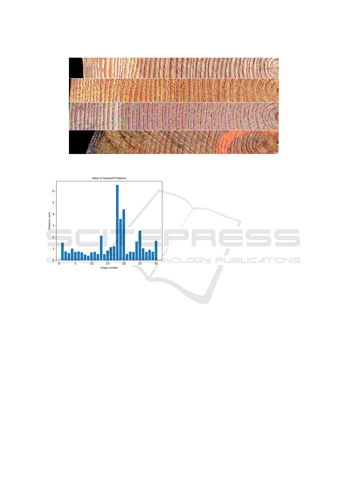
Figure 10: Four examples of extracted sub-images to assess the segmentation quality. Blue lines are ground truth, red lines

are predicted boundaries and green lines are boundaries where predicted and ground truth match.

Figure 11: Mean Hausdorff Distance for 30 sub-images

with ground truths.

images similar to Figure 10 most-left and left than

most-right and right in training set. Neural network

learned to detect edges but struggled to detect bound-

aries when there are strong noises. Our method also

struggles to detect such boundaries but, since the ori-

entation is assumed to be known, strong noises are

reduced.

Concerning the bias, it is −0.441 mm for

(Longuetaud et al., 2022) dataset with conﬁdence in-

cluded and −0.034 mm without. Deep learning ap-

proach seems to overestimate the width. This could

be due to not well-segmented tree rings. It detects less

boundaries than our proposed method does (see Fig-

ure 10). Using the conﬁdence map reduces the biais

and sometimes even makes it negative. One explana-

tion is that tree rings are more visible outwards the

pith and are well-segmented, but those tree rings have

smaller width than those close to the pith. This also

explains why the bias is always negative.

Furthermore, these values should be considered in

light of how the ground truth was obtained, for at least

(Longuetaud et al., 2022) dataset. The ground truth

was obtained from 4 orthogonal directions, while in

our method, we potentially consider all possible di-

rections. Additionally, the resolution of the processed

images is not the same as that used for the ground

truth. We cannot be more precise than a certain dis-

tance due to the image resolution. On average, one

pixel is equivalent to 0.21 mm, meaning that a varia-

tion of one pixel results in a variation of around 3.75%

from the ground truth.

Nonetheless, all these values are encouraging and

support our method for both tree ring detection and

conﬁdence map. Some reﬁnements should lead to

better estimation.

As we already said, a good estimation of tree ring

width does not imply a well delineation of tree rings.

For this, we process two further measurements. How-

ever, having ground truth for the entire dataset is very

challenging. Therefore, we have selected 30 sub-

images for segmentation assessment. These subim-

ages are in core-style, i.e. we select one of the four

directions then from the pith to the outwards (see

Figure 10). Subimages are reoriented in order to al-

ways have the pith on the right. Each subimages has

a height of 128 pixels. The ground truth is shown

in blue while the detected tree rings is in red. Fi-

nally, in green, pixels where the estimation matches

the ground truth are highlighted.

Figure 11 shows the mean Hausdorff distance de-

picted in Equation 4 for these 30 sub-images. The

resulting mean is 1.349 mm, that is close the value of

RMSE previously obtained. It is encouraging for the

future works. Nevertheless, as already mentioned, the

mean tree ring width of the whole image is not nec-

essarily a great indicator of a good detection. For in-

ICPRAM 2024 - 13th International Conference on Pattern Recognition Applications and Methods

858

stance, the image with highest d

hauss

(a value of 6.523

mm) is obtained for the last image in Figure 10 and it

is not the image with the highest mean tree ring width

(a value of 11.988 mm). Results show that introduc-

ing a conﬁdence map is relevant.

5 CONCLUSIONS

A new framework is presented by combining a direc-

tional ﬁlter to detect tree rings and a conﬁdence map

to perform measurements on detected tree rings. The

method works on untreated cross-section wood im-

ages. Over the experiments, it achieves a RMSE of

0.830 mm for the (Longuetaud et al., 2022) dataset,

slightly better than a deep learning method of 1.482

mm. We also obtained great results for Urudendro

dataset (Marichal et al., 2023b) with a RMSE of

14.626 pixels. Note that combining the conﬁdence

map and deep learning offers also great results.

In future works, we will include automatic pith de-

tection, cross-section segmentation, other tree species

and other deep learning methods. We will also adapt

our method to other applications where orientation

plays an important role such as ﬁngerprint images.

REFERENCES

Aydin, O. U., Taha, A. A., Hilbert, A., Khalil, A. A., Gali-

novic, I., Fiebach, J. B., Frey, D., and Madai, V. I.

(2021). On the usage of average hausdorff distance

for segmentation performance assessment: hidden er-

ror when used for ranking. European radiology exper-

imental, 5:1–7.

Chen, L.-C., Zhu, Y., Papandreou, G., Schroff, F., and

Adam, H. (2018). Encoder-decoder with atrous sep-

arable convolution for semantic image segmentation.

In Proceedings of ECCV, pages 801–818.

Conner, W. S., Schowengerdt, R. A., Munro, M., and

Hughes, M. K. (1998). Design of a computer vi-

sion based tree ring dating system. In IEEE South-

west Symposium on Image Analysis and Interpretation

(Cat. No. 98EX165), pages 256–261.

Decelle, R., Ngo, P., Debled-Rennesson, I., Mothe, F., and

Longuetaud, F. (2021). Digital straight segment ﬁlter

for geometric description. In International Confer-

ence on Discrete Geometry and Mathematical Mor-

phology, pages 255–268.

Decelle, R., Ngo, P., Debled-Rennesson, I., Mothe, F., and

Longuetaud, F. (2022). Ant colony optimization for

estimating pith position on images of tree log ends.

Image Processing On Line, 12:558–581.

Decelle, R., Ngo, P., Debled-Rennesson, I., Mothe, F., and

Longuetaud, F. (2023). Light u-net with a new mor-

phological attention gate model application to analyse

wood sections. In ICPRAM 2023.

Fabija

nska, A. and Danek, M. (2018). Deepdendro–a tree

rings detector based on a deep convolutional neural

network. Computers and electronics in agriculture,

150:353–363.

Gillert, A., Resente, G., Anadon-Rosell, A., Wilmking, M.,

and von Lukas, U. F. (2023). Iterative next bound-

ary detection for instance segmentation of tree rings

in microscopy images of shrub cross sections. In Pro-

ceedings of IEEE CVFPR, pages 14540–14548.

Gonzalez, R. C. (2009). Digital image processing. Pearson

education india.

He, K., Zhang, X., Ren, S., and Sun, J. (2016). Deep resid-

ual learning for image recognition. In Proceedings of

IEEE CCVPR, pages 770–778.

Kurdthongmee, W. (2020). A comparative study of the ef-

fectiveness of using popular dnn object detection al-

gorithms for pith detection in cross-sectional images

of parawood. Heliyon, 6(2).

Laggoune, H., Guesdon, V., et al. (2005). Tree ring analy-

sis. In IEEE Canadian Conference on Electrical and

Computer Engineering, pages 1574–1577.

Longuetaud, F., Pot, G., Mothe, F., Barthelemy, A., Decelle,

R., Delconte, F., Ge, X., Guillaume, G., Mancini, T.,

Ravoajanahary, T., et al. (2022). Traceability and qual-

ity assessment of douglas ﬁr (pseudotsuga menziesii

(mirb.) franco) logs: the treetrace douglas database.

Annals of Forest Science, 79(1):1–21.

Makela, K., Ophelders, T., Quigley, M., Munch, E., Chit-

wood, D., and Dowtin, A. (2020). Automatic tree

ring detection using jacobi sets. arXiv preprint

arXiv:2010.08691.

Marichal, H., Passarella, D., Lucas, C., Profumo, L., Casar-

avilla, V., Rocha Galli, M. N., Ambite, S., and Ran-

dall, G. (2023a). UruDendro: An Uruguayan Disk

Wood Database For Image Processing.

Marichal, H., Passarella, D., and Randall, G. (2023b). Cs-

trd: a cross sections tree ring detection method. arXiv

preprint arXiv:2305.10809.

Norell, K. and Borgefors, G. (2008). Estimation of pith po-

sition in untreated log ends in sawmill environments.

Computers and Electronics in Agriculture, 63(2):155–

167.

Pol

cek, M., Arizpe, A., H

uther, P., Weidlich, L., Steindl,

S., and Swarts, K. (2023). Automation of tree-ring de-

tection and measurements using deep learning. Meth-

ods in Ecology and Evolution, 14(9):2233–2242.

Russakovsky, O., Deng, J., Su, H., Krause, J., Satheesh,

S., Ma, S., Huang, Z., Karpathy, A., Khosla, A.,

Bernstein, M., Berg, A. C., and Fei-Fei, L. (2015).

ImageNet Large Scale Visual Recognition Challenge.

International Journal of Computer Vision (IJCV),

115(3):211–252.

Venkatesh, M. and Seelamantula, C. S. (2015). Directional

bilateral ﬁlters. In Proceeding of IEEE ICASSP, pages

1578–1582.

Wimmer, G., Schraml, R., Hofbauer, H., Petutschnigg, A.,

and Uhl, A. (2021). Two-stage cnn-based wood log

recognition. In International Conference on Compu-

tational Science and Its Applications, pages 115–125.

Directional Filter for Tree Ring Detection

859