Counting Red Blood Cells in Thin Blood Films: A Comparative Study

Alan Klinger Sousa Alves

1 a

and Bruno Motta de Carvalho

2 b

Instituto Federal de Educac¸

ao, Ci

encia e Tecnologia do Rio Grande do Norte - Campus Nova Cruz,

Av. Jos

e Rodrigues de Aquino Filho, Nova Cruz, Brazil

Departamento de Inform

atica e Matem

atica Aplicada, Universidade Federal do Rio Grande do Norte,

Rua Cel. Jo

ao Medeiros, Natal, Brazil

Keywords:

Malaria, Computer Vision, RBC Counting.

Abstract:

Malaria is a disease caused by a parasite that is transmitted to humans through the bites of infected mosquitoes.

There were an estimated 247 million cases of malaria in 2021, with an estimated number of 619,000 deaths.

One of the tasks in diagnosing malaria and prescribing the correct course of treatment is the computation of

parasitemia, that indicates the level of infection. The parasitemia can be computed by counting the number of

infected Red Blood Cells (RBCs) per µL or the percentage of infected RBCs in 500 to 2,000 RBCs, depending

on the used protocol. This work aims to test several techniques for segmenting and counting red blood cells

on thin blood ﬁlms. Popular methods such as Otsu, Watershed, Hough Transform, combinations of Otsu with

Hough Transform and convolutional neural networks such as U-Net, Mask R-CNN and YOLO v8 were used.

The results obtained were compared with two other published works, the Malaria App and Cell Pose. As a

result, one of our implemented methods obtained a higher F1 score than previous works, especially in the

scenario where there are clumps or overlapping cells. The methods with the best results were YOLO v8 and

Mask R-CNN.

1 INTRODUCTION

Malaria is a disease caused by a parasite of the genus

Plasmodium and it is transmitted by some mosquitoes

of the genus Anopheles (Giacometti et al., 2021). The

main method for diagnosing malaria infections is op-

tical microscopy (Organization et al., 2021). In order

to have the right course of treatment, it is necessary

to determine the specie of the plasmodium, the stage

of the disease and parasitemia of the sample. Thus,

it is important to make a proper estimate, as both an

overestimation or an underestimation can be equally

harmful (Eziefula et al., 2012). The parasitemia is

computed as a percentage of infected Red Blood Cells

(RBCs) relative to the total number of red blood cells

(Organization et al., 2021). Thus, a high accuracy in

the red blood cell counting process is very important

for achieving accurate parasitemia results.

Estimating parasitemia from thin blood ﬁlms has

been addressed in several studies (Rehman et al.,

2018). However, there is still room for improvement,

specially in the case of clumped or overlapped cells

https://orcid.org/0000-0003-2501-4751

https://orcid.org/0000-0002-9122-0257

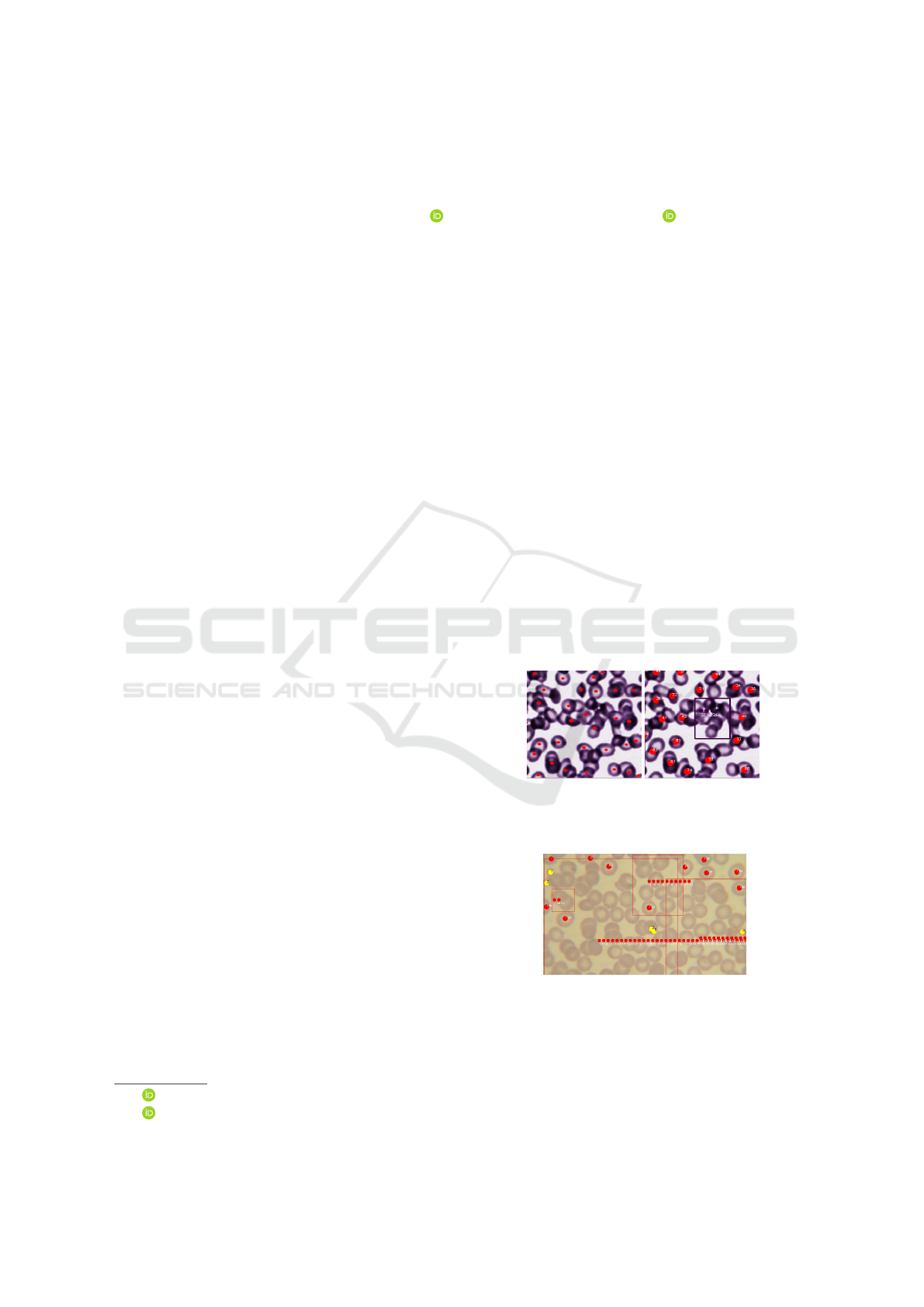
a) Cell Pose b) Malaria App

Figure 1: Both tools present difﬁculty in individually iden-

tifying each RBC in the scenario with overlapped cells.

Figure 2: The Malaria App makes a rectangle around the

cells and then estimates the number of cells in the area. This

estimate may not be very efﬁcient.

(Rehman et al., 2018). Figure 1 shows the result of

the RBC segmentation of two published methods for

the same sample, on the left side, Figure 1a, we have

the segmentation generated by Cell Pose (Stringer

Alves, A. and Motta de Carvalho, B.

Counting Red Blood Cells in Thin Blood Films: A Comparative Study.

DOI: 10.5220/0012455000003657

Paper published under CC license (CC BY-NC-ND 4.0)

In Proceedings of the 17th International Joint Conference on Biomedical Engineering Systems and Technologies (BIOSTEC 2024) - Volume 2, pages 687-694

ISBN: 978-989-758-688-0; ISSN: 2184-4305

687

et al., 2021) and on the right side, Figure 1b, we have

the segmentation from Malaria App (Oliveira, 2019),

Both present poor results in the scenario where the

cells are very close to each other, with the red dots

indicating which cells were identiﬁed. In this case

many cells went unnoticed. This problem is reported

in several other works (Rehman et al., 2018).

In the case of the Malaria App (Oliveira, 2019),

there is still a worst case scenario that can be seen in

the Figure 2, that happens when the algorithm cannot

break down clumps of red blood cells and produces an

estimative of the number of cells in an area marked by

a rectangle. In this case, it is possible that the method

produces a lower quality estimate, with a larger error,

that can affect the computed parasitemia.

The objective of this work is to propose alternate

methods for counting RBCs in thin blood ﬁlms and

analyze their results, in order to obtain more accu-

rate parasitemia estimates. Section 2 presents some

related works while Section 3 brieﬂy describes the im-

plemented methods. Section 4 presents the results and

a discussion about them. Finally, Section 5 presents

our conclusion and suggests future work for this task.

2 RELATED WORK

One of the main related works is the Malaria App

(Oliveira et al., 2018) (Oliveira, 2019), which em-

ployed an adaptive version of the Otsu threshold

(Otsu, 1979) to produce binary images, segmenting

the RBCs from the background. Morphology oper-

ations such as hole ﬁlling, dilation and erosion were

performed to ﬁll up cells and break down connected

cells, these operations are already known and recom-

mended (Wu et al., 2010). Finally, clumps of cells are

identiﬁed and the number of RBCs in each clump are

estimated based on the area and border length of the

clump. The infected cells and white cells are detected

using a Hue, Saturation and value (HSV) ﬁlter, since

the malaria samples are stained with the Giemsa dye.

Another important related work is Cell Pose

(Stringer et al., 2021) which used a generalist ap-

proach through a convolutional neural network based

on an U-Net. Approximately 510 images of mi-

croscopic objects were used for training, but not all

of them are of blood cells. Cell Pose was tested

and compared to other state-of-the-art tools, obtain-

ing results superior to all. The comparisons were

performed against the results produced by Stardist

(Schmidt et al., 2018), Mask R-CNN (He et al., 2017)

(Abdulla, 2017) and the U-Net (Ronneberger et al.,

2015) with two and three classes. A test was carried

out with 111 images similar to our study, and Cell

Pose achieved an accuracy of 93% in the Intersec-

tion Over Union (IoU) metric, while Mask R-CNN

achieved 82% and Stardist achieved 75%.

In another study, (Devi et al., 2018) proposed a

method for detecting infected erythrocytes that uses

Otsu’s thresholding to obtain binary images of the

thin blood samples, followed by a Watershed segmen-

tation. Then, they extracted 54 features that are fed to

several feature selection techniques to remove irrel-

evant data. The selected features are used to train

several different classiﬁers (SVM, k-NN and Naive

Bayes) that are also combined in hybrid classiﬁers.

It is important to note that that method only detects

the infected cells and does not count all the RBCs.

The RBC and white blood cells (WBC) counts are

also important for the diagnosis of other diseases such

as leukemia, allergies, tissue injuries, bronchogenic

infection, anemia and even kidney tumors and lung

diseases (Society, 2023). For this reason, there are

several studies that seek to count RBC or WBC. The

techniques for both are similar, where some of the

techniques being used are based on separation by col-

ors on the Hue, Saturation and Intensity (HSI) color

space or the L*a*b* color space, or on machine learn-

ing techniques such as K-Means, Fuzzy C-Means or

convolutional neural networks (CNNs) (Tran et al.,

2018).

A combination of Ycbcr space Color conversion

was used in conjunction with a circle Hough Trans-

form and watershed algorithm, with this method ob-

taining an accuracy of 90.98% in Acute lymphoblastic

leukemia image database (ALL-IDB) (Yeldhos et al.,

2018). Using the same data set, another work applied

a SegNet obtaining an accuracy rate of 85.50% for

WBC and 82.9% for RBC (Tran et al., 2018).

The network You Only Look Once (YOLO) ver-

sion 2 was also used for WBC detection, achieving

a detection accuracy of 96% (Abas et al., 2021), to

100% (Wang et al., 2018). It is important to note that

the WBC detection problem is simpler than RBC seg-

mentation, as some samples have many objects over-

lapping each other in the latter case.

In this work, we also use convolutional networks

such as the U-Net (Ronneberger et al., 2015) which

has the advantage of producing better results when

working with fewer samples when compared to other

convolutional neural networks (CNNs), the Mask R-

CNN (Abdulla, 2017), which is an extension of a R-

CNN that adds the object mask prediction and the

newest version of the YOLO, the YOLO v8 (Jocher

et al., 2023).

HEALTHINF 2024 - 17th International Conference on Health Informatics

688

3 METHODOLOGY

This work began by obtaining the same data set

used in the Malaria App project (Oliveira, 2019),

then we started with the implementation of tradi-

tional methods that did not use neural networks us-

ing only Python and OpenCV. The data set consists

of 30 samples that were stained with the Giemsa dye

and imaged using a standard optical microscope using

a 1000× zoom, the standard protocol for diagnosing

malaria. The images were originally captured with a

resolution of 2592 × 1944, and reduced to 640 × 480

in our case, since the detection and counting of RBCs

do not need a high resolution image.

Now, we proceed by brieﬂy describing the used

algorithms.

3.1 Otsu

Otsu’s method (Otsu, 1979) is an algorithm for de-

termining an optimal threshold for separating pixels

from an image into two classes. It has been exten-

sively used in its original form and in adaptive ways,

usually by subdividing the image into blocks, thus,

avoiding problems caused by non-uniform illumina-

tion and contrast.

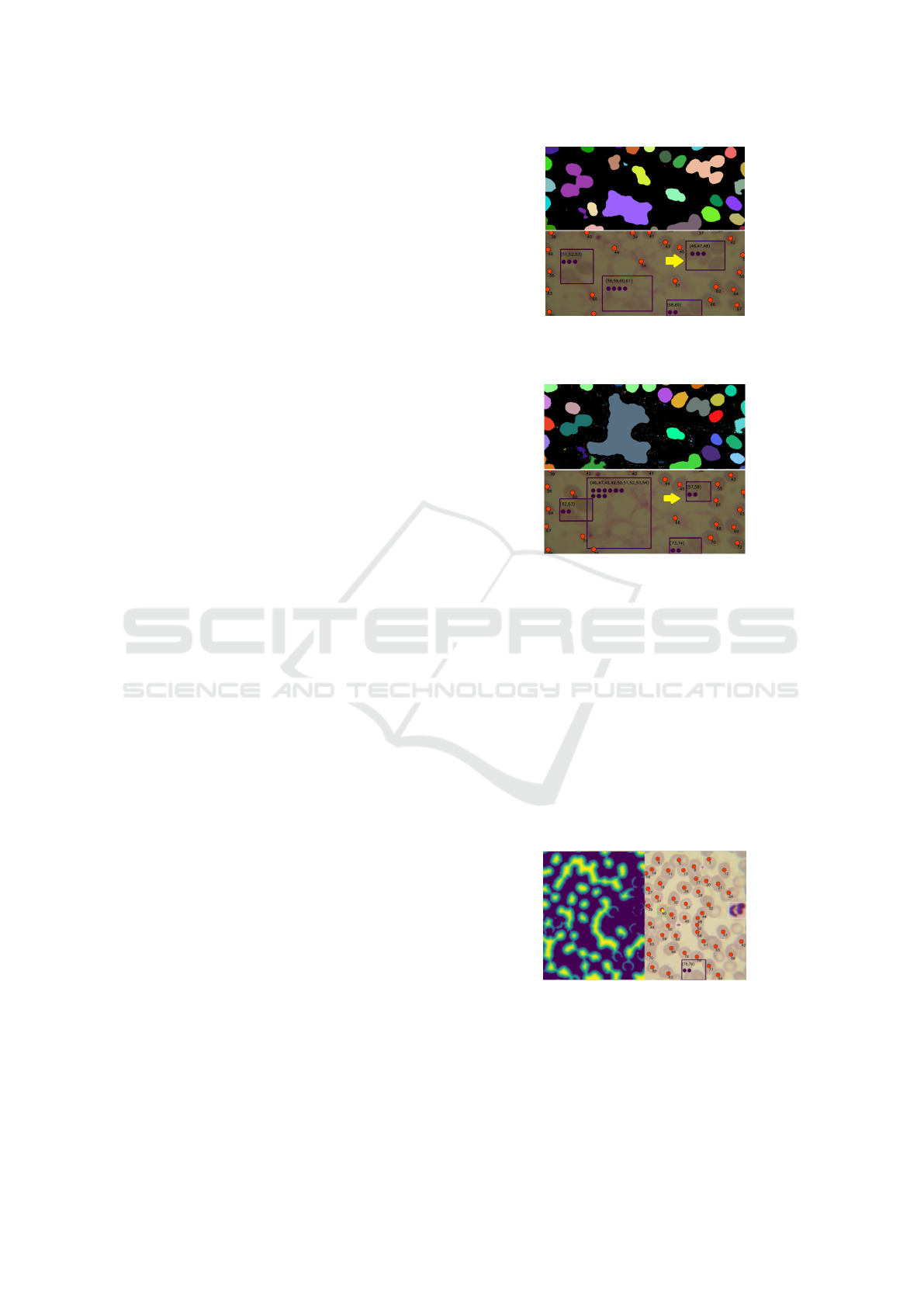
It was noticed that in this method the blurring ﬁl-

ter was bringing together the edges of some cells. It is

possible to see an example of this effect in Figure 3,

we have a group indicated by the yellow arrow with

the wrong estimate, they should have 4 cells but 3

were estimated. In Figure 4, fewer cells were included

in the group, thus, the estimate obtained the correct

answer, in this Figure we have the same method, but

without the blur. In general, even without blurring the

image, this method generates many groups of cells,

which cannot be segmented individually, having to

resort to making an estimate, similar to what was im-

plemented in Malaria App. This estimate can be quite

wrong when the group contains many cells.

In both Figures it is also possible to notice another

problem: this method captures practically any object,

for example, the spot in the center of both Figures 3

and 4 that was identiﬁed as a group of cells, therefore,

this will generate many false positives. In this work

we generate results for Otsu Adaptive, which in the

tables appears labeled as Otsu and for Otsu Adapta-

tive with Gaussian blur, which in the tables appears

labeled as Otsu + Gaussian blur.

3.2 Watershed

The Watershed algorithm views an image as a topo-

graphic surface in which high intensities denote peaks

Figure 3: Segmentation with Otsu + Gaussian blur, the spots

are identiﬁed as cells and the estimation of the group iden-

tiﬁed by the yellow arrow is ﬂawed.

Figure 4: Segmentation with Otsu, the groups of cells iden-

tiﬁed by the yellow arrow became smaller and the estima-

tion improved.

and hills while low intensities denote valleys, and

gradually ﬁlls the valleys until the water from differ-

ent regions merge. Then, an “artiﬁcial dam” is built

between them and determine boundaries between ob-

jects.

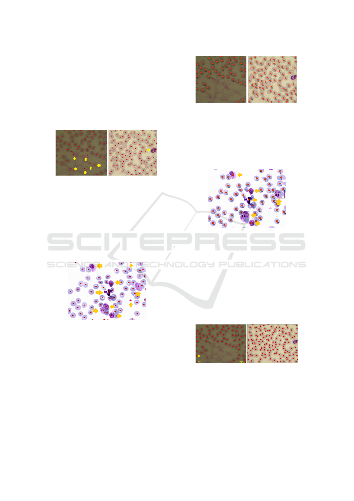
Figure 5 shows the result of the Watershed algo-

rithm, that generates something similar to a relief map

of the image (left) and the RBC labeling on the right.

Note that although some cells appear to be together,

it manages to separate them. One of the problems no-

ticed is that it has difﬁculty ﬁnding cells that are very

clear and in some cases it generates groups of cells.

Figure 5: Watershed segmentation can individually identify

some cells that are very close to each other, but has difﬁculty

identifying very light cells.

Watershed also doesn’t make a good distinction

between sample objects. In Figure 6 with sample C,

we can see 8 false positives.

Counting Red Blood Cells in Thin Blood Films: A Comparative Study

689

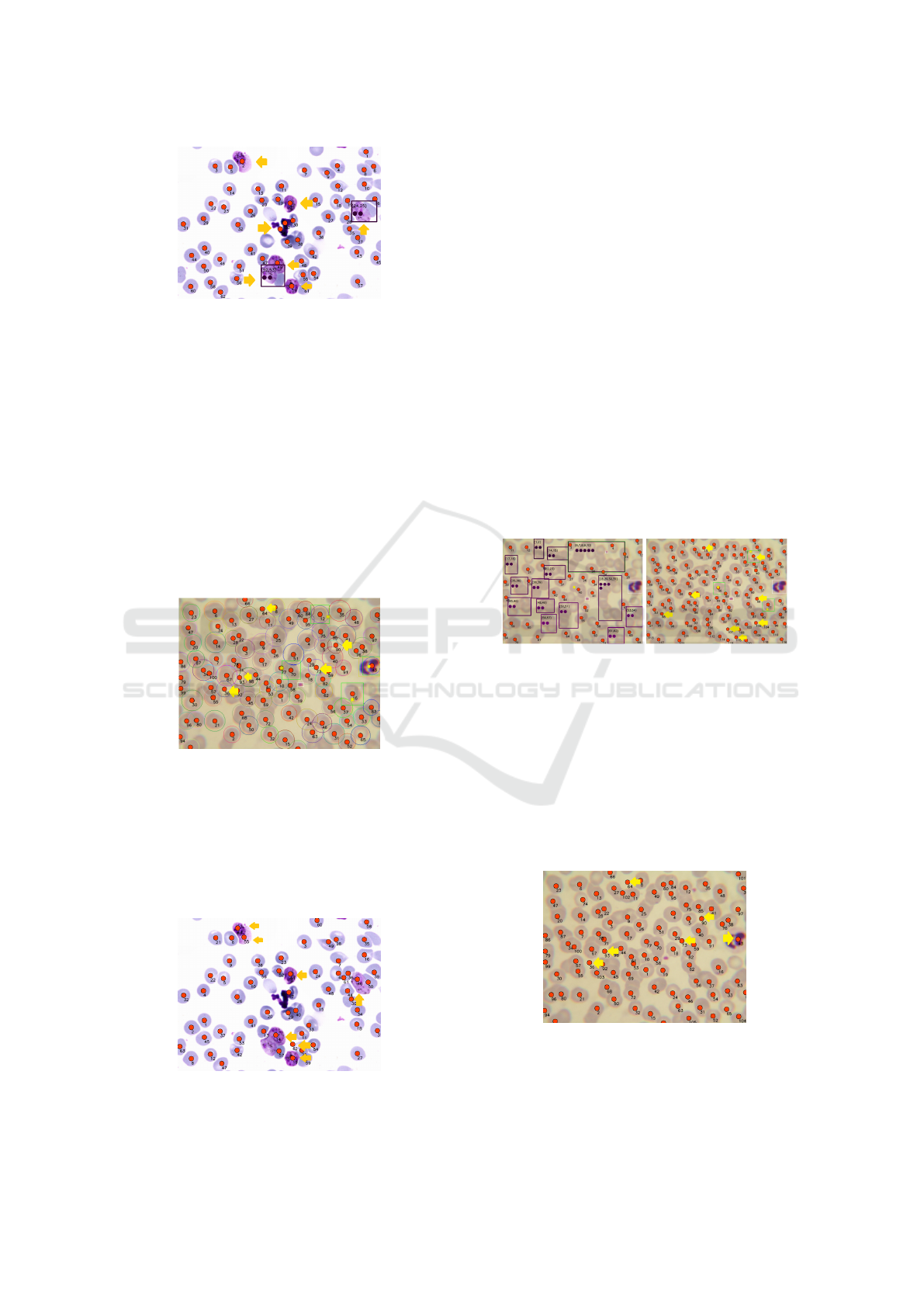
Figure 6: Yellow arrows show incorrect classiﬁcations with

Watershed, any object is incorrectly classiﬁed as a cell.

3.3 Circle Hough Transform

This method uses the circle Hough Transform from

Python’s OpenCV library to identify circles in the

sample. The difﬁculty of the method is the conﬁg-

uration of the parameters. Figure 7 shows the result

of the method with each circle that was found in sam-

ple B, the perceived problem is that this method ﬁnds

circles in places where there are no cells, generating

false positives. We indicate this problem with yel-

low arrows. Furthermore, this method has difﬁculty

capturing cells that are not in an approximate circular

shape.

Figure 7: Empty spaces can be classiﬁed as cells if objects

in the surrounding environment form something like a cir-

cle, the yellow arrows point out these problems.

In Figure 8 we have a sample with 7 false posi-

tives, in which we can observe that the circle Hough

Transform will capture any object that is in a circular

format, making no distinction between contaminated

cells, WBCs and RBCs.

Figure 8: Incorrect classiﬁcation with circle Hough Trans-

form, any circular shaped object is identiﬁed as a cell, as

highlighted by the yellow arrows.

3.4 Otsu + Circle Hough Transform

We noted that the circle Hough Transform and Otsu

could overcome some of each other’s deﬁciencies,

since the circle Hough Transform can identify cells

individually, even if they are very close, while Otsu

can identify cells that are in different formats, so we

decided to test two methods that would unite Otsu and

the circle Hough Transform.

The ﬁrst method would be, after using Otsu, in-

stead of trying to make an estimate to identify the

number of cells in the groups that could not be sep-

arated, use circle Hough Transform to break down

the groups of cells generated. In this way we imple-

mented Otsu + Hough 1, whose result for a sample

can be seen in Figure 9. The Figure 9a shows that

Otsu created several groups, while in Figure 9b there

is the same sample with the result generated by Otsu

+ Hough 1. there, it is possible to see that all groups

were individually segmented with only 8 false posi-

tives indicated by the yellow arrows.

a) Otsu b) Otsu + Hough 1

Figure 9: Segmentation with Otsu + Hough 1, ﬁgure (a)

shows the result of Otsu, ﬁgure (b) shows the result of Otsu

after breaking the cell groups with the circle Hough Trans-

form. Yellow arrows highlight false positives.

The second method would simply be to combine

the Otsu result with circle Hough Transform, we call

this method Otsu + Hough 2, this second method gen-

erates fewer false positives, but ﬁnds fewer cells than

the previous method. A result of its use can be seen

in Figure 10.

Figure 10: Segmentation with Otsu + Hough 2, this combi-

nation is the simple sum of the results of the two methods,

consequently there will be errors present in both methods.

Yellow arrows highlight false positives.

HEALTHINF 2024 - 17th International Conference on Health Informatics

690

3.5 Mask R-CNN

Mask R-CNN (Abdulla, 2017) was the slowest

method, with its execution taking about 1 minute and

30 seconds to segment just one sample. This time

does not preclude its use, but it is important to high-

light it. This network obtained good results, with two

examples being shown on Figure 11. It is possible to

see that it generates few false positives and does not

generate groups of cells.

a) Sample A b) Sample B

Figure 11: Mask R-CNN was not able to accurately differ-

entiate cells from spots and others objects. Yellow arrows

highlight problems.

Despite the good results with images with clumps

of cells, Mask R-CNN also presented a problem: it

considers most objects as RBCs. In sample C pre-

sented in Figure 12, it is possible to observe at least

11 objects that were erroneously classiﬁed as RBCs.

The problem occurs in most samples and can also be

seen in Figure 11.

Figure 12: Wrong classiﬁcation with Mask R-CNN, this

neural network is also not capable of differentiating cells

from other objects in the samples. Yellow arrows highlight

problems.

3.6 U-Net

U-Net is also a convolutional network, with a big ad-

vantage that it is fast to train and requires fewer im-

ages to obtain a good result when compared to other

CNNs. Figure 13 exempliﬁes its use with two sam-

ples. It was one of the only methods that did not

generate false positives, managing to precisely differ-

entiate the cells from spots. In Figure 13b, does not

generate false positives, however, it ﬁnds fewer cells

than actually exist in the image.

a) Sample A b) Sample B

Figure 13: For these samples, U-Net can differentiate spots

and others objects from cells.

Like Mask R-CNN, U-Net also captures many ob-

jects such as RBCs, but in smaller quantities, Figure

14 is the same sample as Figure 12 but with only 6

false positives. Just by looking at Figure 13 it would

not be possible to observe this problem.

Figure 14: U-Net cannot differentiate cells from other ob-

jects when they are very similar to them. False positives are

indicated with yellow arrows.

3.7 YOLO v8

The version 8 of YOLO at the moment is the latest

one of this convolutional network. This network had

a reasonable training time, but the segmentation exe-

cution takes less than 1 second. Figure 15 shows that

it generated some false positives in sample A, but it

was the only method that found all RBCs in the sam-

ple B.

a) Sample A b) Sample B

Figure 15: The segmentation with YOLO v8 made only a

few false positives in the image (a) highlighted by the yel-

low arrows and managed to ﬁnd all the red blood cells in

the image (b).

Unlike the two previous convolutional networks,

YOLO v8 correctly classiﬁes most objects, an exam-

ple can be seen in Figure 16, where there are no false

positives.

Counting Red Blood Cells in Thin Blood Films: A Comparative Study

691

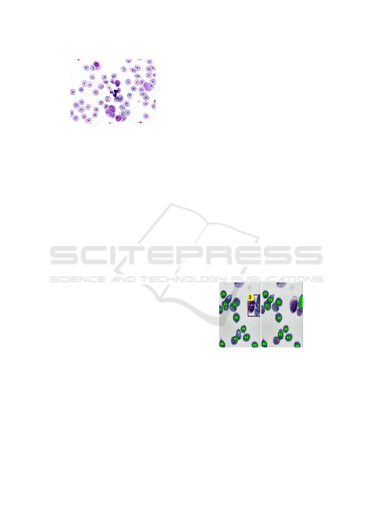
Figure 16: Good classiﬁcation with YOLO v8. It was pos-

sible to differentiate even cell-like objects.

4 EXPERIMENTS

In this session we describe the experiments per-

formed, the metrics used for comparing the results

and present the results.

After testing traditional algorithms for segmenta-

tion, we started testing with convolutional networks

such as U-Net, Mask R-CNN and YOLO v8. In order

to train a more general model, an additional 400 mi-

croscopic images were obtained, of which 100 would

be used only for validation and comparison of the

methods. With these 330 images, data augmentation

was carried out with rotations and mirroring, generat-

ing 2,860 images. The experiments were performed

on a computer equipped with 40 Intel Xeon E5-2660

CPUs and with 64GB of RAM.

Resolutions of 256, 384, 416, 512 and 1024 were

tested for the convolutional networks, however data

will only be presented for the resolutions that pro-

vided the best results.

The U-Net took 28 hours to train for 1,500 epochs

using Tensorﬂow (Abadi et al., 2015), Adam opti-

mizer (Kingma and Ba, 2014) and binary cross en-

tropy as the loss function with the resolution of 256 ×

256. A total of 2,145 images were used for training

and 715 for validation.

For the Mask R-CNN training, we used the same

parameters used in U-Net, 2,145 images for train-

ing and 715 for validation, the best resolution was

1024× 1024. The initial weights were the same as the

ones used on ImageNet, and we used 20 epochs for

the net head and 40 epochs for the other layers. Each

epoch had 100 steps of training, using the ResNet50’s

backbone. The whole training took approximately 6

days.

For the YOLO v8, we used 1,425 images for train-

ing, 804 for validation and 631 for testing. The train-

ing used 2,000 epochs with a batch size of 25 and the

best resolution was 512 × 512, in about 59 hours.

4.1 Comparing Results

Our objective was not to perform an exact segmen-

tation, but rather a precise count of the RBCs in the

sample, for this reason, we did not use the Intersec-

tion over Union (IoU) metric.

We created a tool to compare the evaluated image

and the ground truth, based on the position of each

RBC. All segmentation algorithms mark each RBC

with a red circle, the comparison tool searches for

these circles, comparing the position of each one with

the closest RBC to the same position in the ground

truth. When an RBC is found in the same position

in both the ground truth and the evaluated image, a

green circle is made above and a number is added, so

that it is possible to check exactly whether the RBC

in that position corresponds to the RBC in the same

position in the other image. This comparison can be

seen in Figure 17, where on the left side (a) we have

the image being evaluated and on the right side (b) we

have the ground truth.

Some algorithms, such as the Malaria App or Wa-

tershed, generate groups of cells and make an esti-

mate for each group. In these cases, a yellow square is

added with the count of the group’s RBCs in the eval-

uated image, the example can be seen in Figure 17(a),

where we have 1 purple rectangle with the count high-

lighted in a yellow square and in the ground truth im-

age the RBCs within the group area are painted light

green, which can also be seen in Figure 17(b).

a) Malaria App b) Ground truth

Figure 17: (a) Results from (Oliveira, 2019) . (b) Ground

truth image, dark green circles mark cells that were cor-

rectly identiﬁed, the light green circles in identify the cells

that were “extracted” from RBC groups, while the smaller

red circles identify the cells that were not detected.

Therefore, the red circles that remain in the im-

age being evaluated are considered false positives and

those that remain in the ground truth image are false

negatives. Additionally, a 50px border was created

around the image to avoid considering RBCs that are

very close to the edge, because the count made by an

expert would not evaluate these RBCs as they are only

partially seen.

HEALTHINF 2024 - 17th International Conference on Health Informatics

692

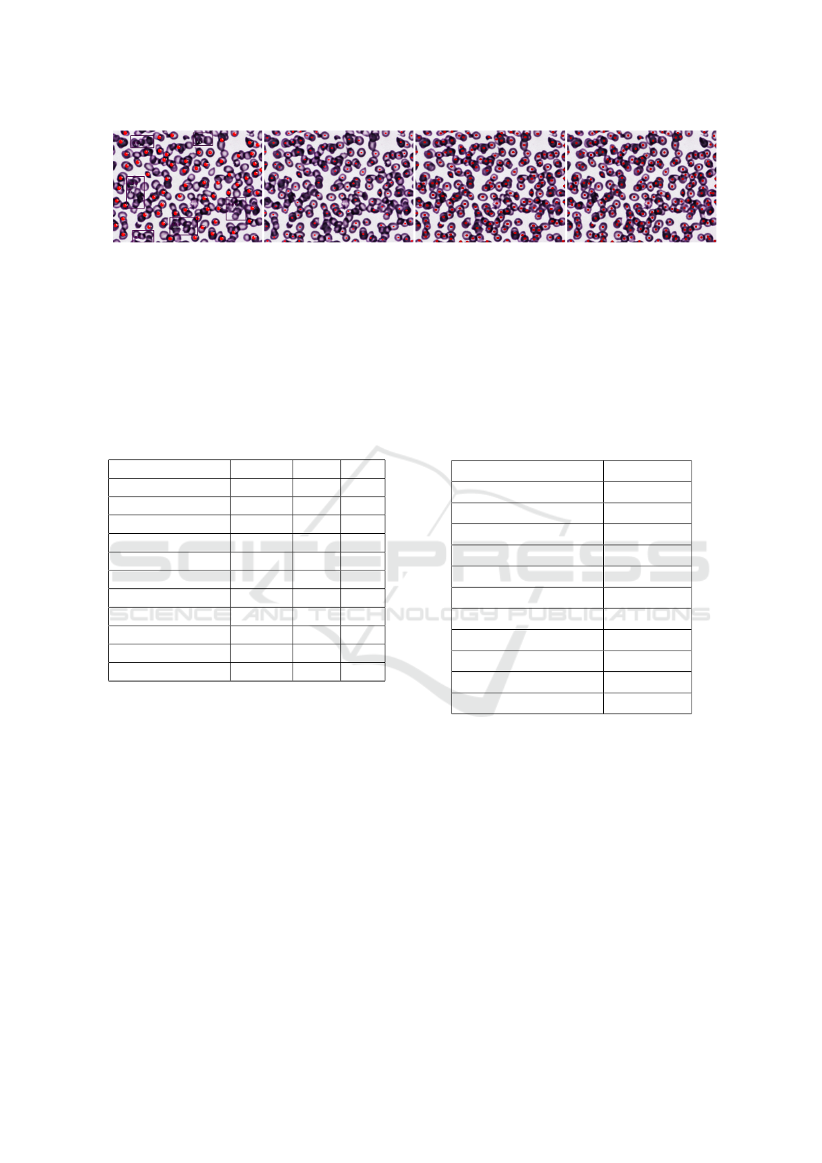
(a) Malaria App (b) Cell Pose (c) R-CNN (d) YOLO v8

Figure 18: Segmentation of a complex sample with 199 RBCs: Malaria App found 84 RBCs, Cell Pose found 113 RBCs,

Mask R-CNN found 172 RBCs and YOLO v8 found 183 RBCs.

4.2 Results

As most methods only took average execution times

between 0.5 and 1.5 seconds per sample, we consider

the time differences as negligible and do not report on

them. Table 1 presents the precision, recall and F1

scores accuracies for all methods tested.

Table 1: Precision, recall and F1 scores.

Method name Precision Recall F1

Hough Transform 0.928 0.817 0.861

Otsu + Gaussian blur 0.898 0.763 0.817

OTSU + Hough 1 0.869 0.887 0.872

OTSU + Hough 2 0.907 0.874 0.886

OTSU 0.902 0.771 0.824

Mask R-CNN 0.919 0.980 0.948

U-Net 0.916 0.842 0.873

Watershed 0.895 0.904 0.894

YOLO v8 0.942 0.976 0.958

Malaria App 0.897 0.842 0.862

Cell Pose 0.936 0.943 0.936

Among the methods tested by us, YOLO v8 ob-

tained the best result in precision and F1 score (0.942)

and (0.958) respectively, followed by circle Hough

Transform with the second highest precision (0.928)

and Mask R-CNN with the second best F1 score

(0.948). Regarding Recall, Mask R-CNN obtained

the best result (0.980), followed by YOLO v8 (0.976).

However, we have to emphasize that the para-

sitemia computation is an easier task than the clas-

siﬁcation task which we are reporting. In the count-

ing task, a false positive and a false negative in the

same sample cancel each other, while in the classiﬁ-

cation task, they count as two errors. Therefore, we

present Table 2 that shows the average percentage of

errors for each implemented method. The errors are

counted in a simpler way: if in the sample there are

10 cells and the algorithm identiﬁed 12 or 8 the er-

ror will be 2. To calculate this percentage, the dif-

ference between the expected count for each sample

and the count carried out by each method was com-

puted, and only then the percentage of this difference

was calculated. According to Table 2, of the methods

tested by us, YOLO v8 managed to have the best error

average with just 5.02% followed by Mask R-CNN

(8.28%), while Malaria App had an average error rate

of 11.22% and Cell Pose had an error rate of 6.81%.

Table 2: Methods error percentage average.

Method Percent error

Circle Hough Transform 15.539

Otsu + Gaussian blur 18.066

Otsu + Hough 1 13.659

Otsu + Hough 2 10.754

Otsu 18.375

Mask R-CNN 8.281

U-Net 11.461

Watershed 10.596

YOLO v8 5.025

Malaria App 11.220

Cell Pose 6.812

In simple samples, most methods present a good

result, and the big difference occurs in samples with

clumped or overlapped cells. Figure 18 presents the

result of segmentation by the two published methods

and the two best methods implemented by us, in one

of the more challenging samples. This sample has

199 RBCs, while Malaria App found only 84 and

Cell Pose found 113, our Mask R-CNN and YOLO

v8 found 172 and 183 respectively.

Cell Pose presents an smaller percent error value

than Mask R-CNN because most of the samples used

in this study are simple. If the majority were more

complex, the Mask R-CNN’s percent error would

probably be smaller than Cell Poses’s percent error.

Counting Red Blood Cells in Thin Blood Films: A Comparative Study

693

5 CONCLUSIONS

The results show the YOLO v8 and Mask R-CNN

as the most accurate ones. The big difference be-

tween these two methods compared to Malaria App

and Cell Pose is in dealing with clumped and over-

lapped RBCs, in which cases both tools present lower

accuracies than YOLO v8 and Mask R-CNN.

As future work, we intend to train convolution

networks to deal speciﬁcally with the problem of

clumped groups of RBCs, the main problem in this

task. Moreover, we believe that the problem may

be simpliﬁed with a better designed pre-processing

phase, with more robust hole ﬁlling and cell separa-

tion procedures. This approach will also be further

investigated.

To have an even more generic CNN, we could add

more images to the training dataset. The difﬁculty lies

in obtaining and labeling each image, as it is a time-

consuming process. Furthermore, other datasets will

need to be created to identify other diseases, so the

labeling process needs to be improved. So, as we al-

ready have a CNN capable of identifying RBCs, we

can use the prediction result as a starting point to la-

bel more samples in a semi-automatic approach, dras-

tically reducing the labeling time.

REFERENCES

Abadi, M., Agarwal, A., Barham, P., et al. (2015). Tensor-

Flow: Large-scale machine learning on heterogeneous

systems. Software available from tensorﬂow.org.

Abas, S. M., Abdulazeez, A. M., and Zeebaree, D. (2021).

A yolo and convolutional neural network for the de-

tection and classiﬁcation of leukocytes in leukemia.

Indones. J. Electr. Eng. Comput. Sci, 25(1).

Abdulla, W. (2017). Mask R-CNN for object detection and

instance segmentation on keras and tensorﬂow. https:

//github.com/matterport/Mask RCNN.

Devi, S. S., Roy, A., Singha, J., Sheikh, S. A., and Laskar,

R. H. (2018). Malaria infected erythrocyte classiﬁ-

cation based on a hybrid classiﬁer using microscopic

images of thin blood smear. Multimed. Tools Appl.,

77(1):631–660.

Eziefula, A. C., Gosling, R., Hwang, J., Hsiang, M. S.,

Bousema, T., Von Seidlein, L., and Drakeley, C.

(2012). Rationale for short course primaquine in

africa to interrupt malaria transmission. Malaria J.,

11:1–15.

Giacometti, M., Milesi, F., Coppadoro, P. L., Rizzo, A., Fa-

giani, F., Rinaldi, C., Cantoni, M., Petti, D., Albisetti,

E., Sampietro, M., et al. (2021). A lab-on-chip tool

for rapid, quantitative, and stage-selective diagnosis

of malaria. Adv. Sci., page 2004101.

He, K., Gkioxari, G., Doll

ar, P., and Girshick, R. (2017).

Mask R-CNN. In Proceedings of the ICCV, pages

2961–2969.

Jocher, G., Chaurasia, A., and Qiu, J. (2023). YOLO by

Ultralytics.

Kingma, D. P. and Ba, J. (2014). Adam: A

method for stochastic optimization. ArXiv preprint

arXiv:1412.6980.

Oliveira, A. D., Carvalho, B. M., Prats, C., Espasa, M.,

i Prat, J. G., Codina, D. L., and Albuquerque, J.

(2018). An automatic system for computing malaria

parasite density in thin blood ﬁlms. In Progress in Pat-

tern Recognition, Image Analysis, Computer Vision,

and Applications, pages 186–193. Springer Interna-

tional Publishing.

Oliveira, A. D. d. (2019). MalariaApp: Um sistema de

baixo custo para diagn

ostico de mal

aria em l

aminas

de esfregac¸o sangu

ıneo usando dispositivos m

oveis.

PhD thesis, Universidade Federal do Rio Grande do

Norte.

Organization, W. H. et al. (2021). Who guideline for

malaria, 13 july 2021. Technical report, World Health

Organization.

Otsu, N. (1979). A threshold selection method from gray-

level histograms. IEEE Trans. on Syst. Man Cybern.,

9(1):62–66.

Rehman, A., Abbas, N., Saba, T., Mehmood, Z., Mah-

mood, T., and Ahmed, K. T. (2018). Microscopic

malaria parasitemia diagnosis and grading on bench-

mark datasets. Mic. Res. Tech., 81(9):1042–1058.

Ronneberger, O., Fischer, P., and Brox, T. (2015). U-

Net: Convolutional networks for biomedical image

segmentation. In Pro. of MICCAI, pages 234–241.

Springer.

Schmidt, U., Weigert, M., Broaddus, C., and Myers, G.

(2018). Cell detection with star-convex polygons. In

Proc. of MICCAI, pages 265–273. Springer.

Society, C. C. (2023). Complete blood count (CBC). https:

//cancer.ca/en/treatments/tests-and-procedures/co

mplete-blood-count-cbc#ixzz5JmJ8jOk9. Accessed:

2023-08-28.

Stringer, C., Wang, T., Michaelos, M., and Pachitariu, M.

(2021). Cellpose: A generalist algorithm for cellular

segmentation. Nat. Methods, 18(1):100–106.

Tran, T., Kwon, O.-H., Kwon, K.-R., Lee, S.-H., and Kang,

K.-W. (2018). Blood cell images segmentation using

deep learning semantic segmentation. In Proc. of the

ICECE, pages 13–16. IEEE.

Wang, X., Xu, T., Zhang, J., Chen, S., and Zhang, Y.

(2018). So-yolo based wbc detection with fourier

ptychographic microscopy. IEEE Access, 6:51566–

51576.

Wu, Q., Merchant, F., and Castleman, K. (2010). Micro-

scope Image Processing. Elsevier.

Yeldhos, M. et al. (2018). Red blood cell counter using

embedded image processing techniques. Res. Rep., 2.

HEALTHINF 2024 - 17th International Conference on Health Informatics

694