Neural Population Decoding and Imbalanced Multi-Omic Datasets

for Cancer Subtype Diagnosis

Charles Theodore Kent

, Leila Bagheriye

and Johan Kwisthout

School of Artificial Intelligence, Radboud Universiteit, Houtlaan 4, Nijmegen, Netherlands

Donders Institute for Brain, Cognition & Behaviour, Radboud Universiteit, Houtlaan 4, Nijmegen, Netherlands

Keywords: Cancer Diagnosis, Multi-Omics, Population Decoding, Spiking Neural Networks, Winner-Take-All,

Hierarchical Bayesian Network, Self-Organising Maps.

Abstract: Recent strides in the field of neural computation has seen the adoption of Winner-Take-All (WTA) circuits to

facilitate the unification of hierarchical Bayesian inference and spiking neural networks as a neurobiologically

plausible model of information processing. Current research commonly validates the performance of these

networks via classification tasks, particularly of the MNIST dataset. However, researchers have not yet

reached consensus about how best to translate the stochastic responses from these networks into discrete

decisions, a process known as population decoding. Despite being an often underexamined part of SNNs, in

this work we show that population decoding has a significant impact on the classification performance of

WTA networks. For this purpose, we apply a WTA network to the problem of cancer subtype diagnosis from

multi-omic data, using datasets from The Cancer Genome Atlas (TCGA). In doing so we utilise a novel

implementation of gene similarity networks, a feature encoding technique based on Kohoen’s self-organising

map algorithm. We further show that the impact of selecting certain population decoding methods is amplified

when facing imbalanced datasets.

1 INTRODUCTION

Multi-omics data integration in cancer diagnosis

refers to the integration of information from various

biological "omics" e.g., genomics, transcriptomics,

metabolomics, to provide a more comprehensive

understanding of the molecular landscape of cancer.

Spiking neural networks (SNNs) are a

neurobiologically inspired method of information

processing which aim to solve tasks using plausible

models of neuron dynamics (Yamazaki et al., 2022).

Much like in biological brains, neurons in SNNs are

linked through excitatory and inhibitory connections,

and propagate information via discrete electrical

signals known as spikes (Yamazaki et al., 2022;

Himst et al., 2023). An important feature of SNNs is

that their activations are stochastic (Ma & Pouget,

2009), and so presenting a network with the same

stimulus multiple times will likely result in varying

responses. We can gain more insight into the network

through sampling the distribution of responses when

presenting a stimulus over multiple time steps,

simulating exposure for a given length of ‘biological

time’ (Guo et al., 2017). The responses of the network

during this window can be quantified by counting the

number of times each neuron spikes, referred to as a

spike count code (Grün & Rotter, 2010).

Alternatively, some research focuses on the time-

dependent relationship of spiking neurons, for

instance by weighting neuron responses more highly

based on how quickly they fire (Grün & Rotter, 2010;

Shamir, 2009; Beck et al., 2008).

In order to extract information from SNNs, we

examine the spikes generated by a population of

neurons in response to a stimulus. The process of

presenting a stimulus to the network to generate these

spikes is known as population encoding, and

conversely the process of obtaining estimates from

the neuron activity patterns is known as population

decoding (Ma & Pouget, 2009). Together, these two

opposite processes are referred to as population

coding. Population coding can be used in conjunction

with SNNs to gain practical insights into how a

system of spiking neurons tackles the task of learning

(Ma & Pouget, 2009).

Approaching the question from a more theoretical

standpoint, Bayesian inference is hypothesised to be

a key component of information processing within the

Kent, C., Bagheriye, L. and Kwisthout, J.

Neural Population Decoding and Imbalanced Multi-Omic Datasets for Cancer Subtype Diagnosis.

DOI: 10.5220/0012454200003657

Paper published under CC license (CC BY-NC-ND 4.0)

In Proceedings of the 17th International Joint Conference on Biomedical Engineering Systems and Technologies (BIOSTEC 2024) - Volume 1, pages 391-403

ISBN: 978-989-758-688-0; ISSN: 2184-4305

391

brain (Guo et al., 2017), including in areas of

cognition and decision making (Shamir, 2009).

Handling uncertainty when understanding their

environment is critical to the survival of many

organisms, and Bayes’ theorem provides a

biologically plausible framework for the brain’s

probabilistic nature (Kersten et al., 2004). Based on

electrophysiological recordings, neurons appear to

process information in a hierarchical manner, which

can similarly be modelled as hierarchical Bayesian

inference (Lee & Mumford, 2003).

Until recently, research into SNNs and hierarchical

Bayesian models of the brain have remained separated

by the computational complexity of performing exact

inference (Guo et al., 2017). To overcome this

problem, the variational principle can be employed to

decompose the difficult exact inference into an

optimisation problem which is easier to solve (Guo et

al., 2017; Friston, 2010). Following this approach,

spiking neural networks have been able to implement

hierarchical Bayesian models through use of neural

circuits such as the Winner-Take-All (WTA) circuit

(Guo et al., 2017; Nessler et al., 2013). In a WTA

circuit, a layer of excitatory neurons is linked to a

corresponding layer of inhibitory neurons. Whenever

an excitatory neuron fires, an inhibitory signal is

generated in response which resets the neuron

membrane potentials to baseline and updating the

weights of each connection (Himst et al., 2023). When

coupled with the spike-timing dependent plasticity

(STDP) learning rule, this framework enables neurons

to learn structural representations from stimuli in an

unsupervised manner (Himst et al., 2023; Guo et al.,

2017; Nessler et al., 2013).

Utilising this technique, experimental research into

hierarchical Bayesian WTA networks have begun

reporting results on the benchmark dataset MNIST

(Himst et al., 2023; Guo et al., 2017; Diehl & Cook,

2015; Nessler et al., 2013; Querlioz et al., 2013).

Generally, the accuracy of these models on the

MNIST test set is in the range of 80-85%, with some

works (Guo et al., 2017; Diehl & Cook, 2015)

achieving accuracies as high as 95% with an

optimised set of model hyperparameters. Whilst the

reported results are promising and show the potential

applications of WTA networks for real-world

problems, current research shows little consideration

to the significance of population coding in

classification tasks.

One point of contention revolves around the choice

of population decoding method used to turn neuronal

responses into a discrete prediction for classification.

In the vast majority of experiments (Himst et al.,

2023; Guo et al., 2017; Diehl & Cook, 2015; Querlioz

et al., 2013), neurons are assigned to the class for

which they spike most frequently over a given dataset

in an a posteriori fashion. Typically, the responses

used to make this assignment are collected by

presenting the network samples from a training set

(Diehl & Cook, 2015; Nessler et al., 2013; Querlioz

et al., 2013), however in some cases (Himst et al.,

2023; Guo et al., 2017) this step is performed over the

test set instead. Unfortunately, the combination of a

posteriori assignment and utilisation of test set labels

can be shown to lead to high degrees of bias, which

we elaborate on in Section 4.

Beyond data subset selection, there are

discrepancies between population decoding practices

adopted by researchers. By far the most common

approach to population decoding (Himst et al., 2023;

Guo et al., 2017; Diehl & Cook, 2015; Nessler et al.,

2013; Querlioz et al., 2013; Ma & Pouget, 2009) is to

assign each neuron a single label based on the class

of stimulus for which the neuron responds most

highly. Then, upon presentation of a test stimulus, the

responses of each neuron are averaged per class,

before selecting the class with the highest average

firing rate. We term this methodology the class

averaging decoder, and give a full mathematical

description in Section 2.

In Nessler et al. (2013), the population decoding

step is hand-performed by a human supervisor by

examining the weights of the trained model. Whilst

this approach is somewhat reasonable in the context

of MNIST, where it is relatively simple for a human

to discern the correct classification by eye, it clearly

leaves a lot to be desired. Firstly, the process is not

scalable, as some notable experimental results (Guo

et al., 2017; Diehl & Cook, 2015) recommend using

many thousands of output neurons for optimal

classification performance. Moreover, not all neurons

in the output population will learn a representation

that is easily recognisable. A given neuron may be

tuned to detect certain sub-features within the image,

be half-way between two distinct classes, or fail to

learn a meaningful representation entirely and have

weights resembling random noise or arbitrary blobs

(Himst et al., 2023; Nessler et al., 2013; Querlioz et

al., 2013). In these cases, human bias can easily creep

into the prediction process, and so a more

mathematically grounded approach is desirable.

Querlioz et al. (2013) use a validation subset of

1,000 “well-identified” images to form their neuron-

class associations. Querlioz et al. (2013) also point

out that the labelling process need not occur

concurrently with training, but can be done at a later

stage. Furthermore, Querlioz et al. (2013) suggests an

avenue for future work could be the coupling of an

BIOINFORMATICS 2024 - 15th International Conference on Bioinformatics Models, Methods and Algorithms

392

SNN to a supervised network to perform the

population decoding step, a concept that we will be

investigating further in this paper.

Notably, in all of the prior discussed approaches,

the population decoding step is treated as separate

from the SNN model. However, it could be argued

that this step must occur somewhere within the brain,

as we are ultimately able to resolve sources of

uncertainty down into concrete choices. The meta-

task of mapping responses from an arbitrarily large

population of neurons down to a single discrete

decision is generally not approached from a

biologically plausible perspective (Ma & Pouget,

2009). As discussed, most methodologies (Himst et

al., 2023; Guo et al., 2017; Diehl & Cook, 2015;

Querlioz et al., 2013) use a running total of the

neuronal responses over each stimulus presented to

the network to determine each neuron’s class. Yet, it

seems implausible for brains to store and update a

counter of every time they have seen a certain class

of stimuli throughout their whole lives, and reference

that counter to make decisions.

A possible alternative to this methodology could be

to incorporate a supervised model to perform the

population decoding step. For instance, a multivariate

logistic regression model requires only the use of a

weight, bias and sigmoid activation function;

components which have each independently been

shown to be neurobiologically plausible (Hao et al.,

2020). Another benefit of logistic regression is that the

model can be trained in an online fashion, updating the

weights and bias upon presentation of each individual

stimulus, and thereby avoiding the necessity of

viewing the entire dataset simultaneously. Whilst this

supervised approach is strictly not biologically

plausible, as the learning and inference steps are not

spike-based (Hao et al., 2020), these factors at least

bring us closer to the desired goal of a complete model

of neural information processing.

One of the key factors to be considered in the

practical application of Bayesian WTA networks is

the role of class imbalance. We posit that the

approaches to population decoding which we have

discussed play a sizeable role in the system’s overall

ability to perform classification, and that class

imbalance has a strong impact on said performance.

Contemporary research primarily focuses on the

MNIST dataset, which has equally balanced class

samples by default, and so issues which arise in this

area have yet to be elucidated. If research is to move

beyond the benchmark domain, handling class

imbalance is a necessity, as innumerable real-world

problems possess this property.

The purpose of this research is to apply an SNN-

based hierarchical Bayesian WTA network to a non-

benchmark dataset, in order to gain further insight into

the implications of selecting various population

decoding methods. The remainder of this paper is

structured as follows. In Section 2, we introduce the

theoretical foundations of population coding in the

context of spiking neural networks, as well as the

definitions for the population decoding strategies we

will test experimentally. In Section 3, the methodology

of the experiments is described in detail. Section 4

contains the results of the aforementioned experiments,

as well as discussions of the insights gained by

practical application of these techniques. Finally,

Section 5 contains concluding remarks, suggested

areas for further research, and provides our

recommendations for future practitioners.

2 POPULATION DECODING

In this section, we provide definitions for the methods

of population decoding which will undergo

experimental evaluation in Section 4. We largely

follow the nomenclature provided by Grün & Rotter

(2010), in which they discuss resolving the ambiguity

of single-trial neuronal responses via population

coding.

Consider an experiment in which a spiking neural

network is presented with a stimulus s from a stimulus

set S. Each stimulus has one associated numeric class

label y



{0,…,C}, where C is the number of possible

classes in y, and s

is the classification for a given

stimulus. The spikes generated by a population of N

neurons in response to presenting a stimulus for a

fixed window of time is recorded. The neural

population response in this time period is quantified

as a vector r = r

,...,r

with dimensionality N, where

is the response of neuron n on a given trial. In this

case we are interested in spike counts, so r

would

therefore be the number of spikes emitted by neuron

n during the trial in the response window. With this

definition of a neural population response, we can

now perform various population decoding methods

with the response array r to associate the response

from a given stimulus s with a predicted classification

label ŷ.

A common strategy (Himst et al., 2023; Guo et al.,

2017; Diehl & Cook, 2015; Nessler et al., 2013;

Querlioz et al., 2013; Ma & Pouget, 2009) for

population decoding is to first associate each output

neuron n with a class label present in ŷ. This

association is created based on the relative strength of

neuronal responses when reacting to stimuli of each

Neural Population Decoding and Imbalanced Multi-Omic Datasets for Cancer Subtype Diagnosis

393

class within the dataset. For each stimulus s presented

to the network, we sum the spike counts r of the

output neurons inside a multi-dimensional array M 

ℤ

N x C

such that





 











(1)

where the sums of spike count responses for each

neuron n are split by class along the c dimension.

Each element M

thus corresponds to the total

amount of times a given neuron spiked for a given

class over the entire stimulus set S.

For each neuron, we can then identify the class

which has the highest spike count over the stimulus

set. In this way, we can experimentally determine a

neuron’s preferred class. We represent this associative

relationship using the vector Z = Z

,...,Z

, with

dimensionality N, defined as:





 







  

(2)

such that each element Z

represents the preferred

class of the corresponding neuron n. For ease of

notation, we can further treat the vector Z akin to a

function, which accepts a parameter n  {1,…, N}

representing the index of a neuron as input, and

returns the preferred class of the neuron at that index.

We denote the neuron’s preferred class as ŷ

  



(3)

From the definition presented in equations 1 & 2,

we can already see there is an implicit assumption that

the stimulus set used to construct Z contains a balanced

number of examples for each class. This is because the

sum of the spike counts is directly proportional to the

amount of times a stimulus of that class is presented to

the network. In datasets with a high degree of class

imbalance, this leads to undesirable behaviour. For

instance, a given neuron may have a far stronger

response to stimuli of one class relative to another - yet

if presented with an overwhelming number of

examples of the “less-prefferred” class, the sum of

spikes for the less-prefferred class will eventually

exceed that of the class with the higher relative spike

response rate. This leads to situations where a neuron

will be assigned a label in Z which is counter to its

observed experimental behaviour. Additional steps

must therefore be taken to rectify this behaviour if we

wish for SNNs to be performant in class-imbalanced

domains.

In the following subsections, we detail the specific

population decoding methods being evaluated in this

research. Additionally, we make note of each

method’s potential robustness to class imbalance as a

natural result of their mathematical construction.

2.1 Winner-Take-All Decoder

For this straightforward population decoding

approach, we designate the neuron with the highest

spike count response the as ‘winner’, then find its

corresponding preferred class in Z to make the final

prediction.

  

(4)

Overall, the simplicity of this methodology does

have significant drawbacks, as each trial is highly

sensitive to variability, and the information from the

responses of all neurons but the most active is

discarded (Ma & Pouget, 2009). In principle, it also

has little resistance to class imbalance, as an unequal

ratio of neuron labels in Z would cause a

disproportionate increase in the likelihood of the

majority class being selected.

2.2 Population Vector Decoder

Another method is to take a sum of the responses per

class, then take the class with the highest amount of

‘votes’ as the network’s prediction (Ma & Pouget,

2009). We split the responses by class in accordance

with the observed preferred class of each neuron Z

such that:





 











  

(5)

This approach is equivalent to the weighted

average shown in (Ma & Pouget, 2009), or is

sometimes referred to as ‘pooling’ the responses of

the neuronal population (Grün & Rotter, 2010). This

is also the approach implemented in Himst et al.

(2023) to achieve their results on the MNIST dataset.

Unfortunately, the population vector decoder is

greatly susceptible to class imbalance, as it is only

concerned with the class-wise sums of responses –

thus incurring the imbalance related problems which

have been discussed above in regards to construction

of the assignment vector Z.

2.3 Class Averaging

In this approach, we take the highest average firing

rate of the neurons per class to determine the

prediction. The sum of spike counts for neurons of

each class is divided by the number of neurons

assigned to that class. Formally,

BIOINFORMATICS 2024 - 15th International Conference on Bioinformatics Models, Methods and Algorithms

394























  

(6)

where Zc is the number of neurons assigned to class

c in the preffered class vector Z.

This is the methodology adopted by Guo et al.

(2017) and Diehl & Cook (2015), and has seen strong

experimental results when applied to the MNIST

dataset. An interesting mechanism at play in this

approach is that, in practice, the distribution of

neurons assigned to each class is proportional to the

class ratio of the stimulus dataset; a property which

we investigate further in our experimental results

Section 4. Due to this property, the class averaging

decoder is inherently more robust to class imbalance

than either of the prior discussed methods.

2.4 Firing Average

Here, we propose a novel method of population

decoding based upon the average firing rate of each

neuron. By subtracting the average firing rate from

the spike counts in the response vector, we can

thereby pay particular attention to neurons which are

abnormally highly active compared to their typical

behaviour. We first compute the vector F = F

,...,F

pertaining to the average firing rate of each neuron

over the a stimulus set of training data:













 



(7)

where |S| is the cardinality of the stimulus set S. We

can subsequently subtract the neuron-wise average to

obtain the final class estimate of the network.





 















  

(8)

This approach is theoretically beneficial in reducing

the impact of ‘over-active’ neurons, which are prone to

firing regardless of the class of the presented stimulus

– effectively acting as a regularization technique.

However, what effect this will have on handling class

imbalance is as yet unknown. Computationally

speaking, calculating the firing average does require an

additional pass over the dataset to calculate the F

vector. Also, utilizing the average spike counts means

the values of the vector F are continuous rather than

discrete, which further distances this methodology

from biological plausibility.

2.5 Logistic Regression

As suggested by Querlioz et al. (2013), a viable

approach to population decoding could be to couple

the SNN to a supervised classification model. To

demonstrate this, we consider a multivariate logistic

regression model to map network responses to

predictions. A variety of other supervised methods

could equally apply here, but as the experimental

section of this research focuses on a case with a

binary target variable, we consider the choice of

logistic regression apt for our purposes. Prediction of

the target from the network response using the trained

logistic regression model is calculated as follows:











 

(9)

where w is the weight vector and b is the bias term.

The training procedure is performed in an online

manner, updating the weights and bias parameters

upon each presentation of a stimulus to the SNN,

rather than over the entire dataset at once after the

SNN training procedure is completed as with the

other population decoding methods.

In regards to the imbalance problem, logistic

regression is reasonably adept at handling skewed

class ratios. In Section 3.1, we apply a logistic

regression model to a heavily imbalanced dataset and

observe strong classification performance (shown in

Figure 1). This result demonstrates the efficacy of the

technique over the original dataset, which suggests it

should likewise be able to handle imbalance in the

role of a population decoder. Additionally,

implementing a supervised model for population

decoding negates the necessity of assigning each

neuron a discrete class. We therefore do not require

the assignment vector Z as in the other described

methods, avoiding the implicit problems with class

imbalance as discussed prior.

3 METHODOLOGY

The dataset we have chosen for practically applying

hierarchical Bayesian WTA networks is from The

Cancer Genome Atlas (TCGA) (Weinstein et al.,

2013). We select the datasets concerning the diagnosis

of breast cancer (BRCA) and kidney renal clear cell

carcinoma (KIRC). The dataset is comprised of multi-

omic features relating to individual patients, including

genomics, methylation and mitochondrial RNA

sequences. Each patient has a corresponding binary

target variable which indicates their cancer diagnosis

status, either positive or negative. Importantly for this

research, there are far fewer examples of positive

diagnoses in both datasets as compared to negative

examples, allowing us to investigate the impact of class

imbalance. Furthermore, the real-world implications of

Neural Population Decoding and Imbalanced Multi-Omic Datasets for Cancer Subtype Diagnosis

395

a false positive versus false negative diagnosis are

worth considering. Patients who receive a false

positive will likely undergo further tests and ultimately

rule out the disease, whereas a false negative could

result in the patient going undiagnosed entirely, which

can have serious ramifications for treatment outcomes.

Therefore, close attention is paid to class-wise

predictive performance throughout the methodological

process.

3.1 Multi-Omic Data

In order to incorporate information from all of the

omic types present in the TCGA dataset, the files for

methylation, genomics and mitochondrial RNA were

combined into a single dataset, with each row

representing one patient mapped to approximately

80,000 omic feature columns. We perform separate

identical processes for the BRCA and KIRC cancer

subtypes. Due to their time-dependent nature, spiking

neural networks generally have a high computational

complexity. Therefore, it is imperative we perform

dimensionality reduction steps upon the dataset in

order to maintain a tractable training regime. In this

vein, we take after the approach of Fatima & Rueda

(2020) and first perform a variance threshold filter

over the data. Any feature with a variance of less than

0.2% is removed. This removes any features with zero

values recorded for more than 80% of samples,

bringing the feature countdown to approximately

20,000 for each cancer subtype.

Feature selection is the next step. There are

numerous possible algorithms which would be

appropriate to apply here; Ang et al. (2015) provides a

rich overview of available methods in the specific

context of genomic feature selection. As we have labels

for our samples, we opt to use supervised feature

selection techniques to best make use of all available

information in the dataset. In particular, the technique

of Minimum Redundancy Maximum Relevancy

(mRMR) (Ding & Peng, 2005) has been selected for

the purposes of this research. mRMR is concerned with

two metrics for feature evaluation; relevancy is a

measure of the mutual information between a feature

and the target, and redundancy measures the mutual

information between features to select mutually

maximally dissimilar genes (Ding & Peng, 2005).

These two scores are then considered with equal

weight to determine the optimal feature subset.

Using mRMR, we calculate the relevancy and

redundancy for each multi-omic feature, and start by

selecting the top 20 scoring features. We then perform

an ablation analysis upon the selected feature set by

training a logistic regression model and sequentially

eliminating the lowest scoring remaining feature,

noting the degradation in predictive performance

each time. In this case we measure performance via

F1-score, a decision which is further explained in

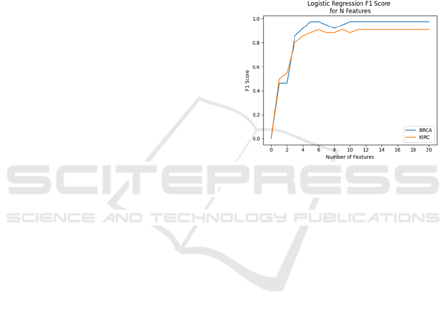
Section 4. The results of this analysis are presented in

Figure 1. Based on these results, we can see that

prediction scores reach their maximum by the

inclusion of the 10 most relevant features for BRCA

and 11 for KIRC. We therefore choose to select the

top 11 features for both cancer subtypes, so that the

pre-processing phase remains identical in either case.

Figure 1: Results of k-folds cross validation for logistic

regression models trained on a range of feature subsets.

Each time the number of features increases, the new feature

being added is the next most important by mRMR score.

3.2 Self-Organising Maps & Gene

Similarity Networks

Bayesian WTA networks of similar design to that

described in this research originate from modelling

the processing systems in the visual cortex. The

design of Bayesian WTA networks typically

incorporates sampling from a Poisson distribution

over a given frame of biological time, as a

representation of the spiking activity of upstream

neuronal firing (Himst et al., 2023; Guo et al., 2017;

Nessler et al., 2013). Therefore, an effective way to

encode information for processing in Bayesian WTA

networks is as a series of binarized images - a 2D grid

where each pixel takes the value of either 0 or 1,

varying across a time dimension. To accomplish this,

the binary images are subsequently encoded into

spike trains (Yamazaki et al., 2022), the process of

which is further described below in Subsection 3.3.

The chosen method for encoding the selected

multi-omic features into an image format is a Self-

Organising Map (SOM) (Kohonen, 1990). This

technique has been applied to TCGA cancer subtype

BIOINFORMATICS 2024 - 15th International Conference on Bioinformatics Models, Methods and Algorithms

396

diagnosis datasets in Fatima & Rueda (2020) with

marked success, and so has been selected for the

purposes of this research. A further aspect of

relevance for this technique is that it has been posited

as a biologically-plausible model of neuron self-

organisation (Kohonen, 1990). As biological

plausibility is likewise a key concern of both

hierarchical Bayesian networks and SNNs in general,

utilising this technique to encode our input data

before presenting it to the network means we can

extend this property to encompass the preprocessing

stage as well.

We employ Kohoen’s Self-Organising Map

algorithm (Kohonen, 1990) to translate each feature

to a node 2D space, where the Euclidean spatial

relationship between nodes encode semantic

information about the input data. The organisation is

done in an unsupervised manner by iteratively

computing the “best matching cell” (Kohonen, 1990)

in accordance with the distance between nodes within

topological neighbourhoods. Each node has an

associated weight vector which is updated

concurrently with its local subset, mimicking lateral

feedback connections in biophysical network models.

The algorithm will run for a set number of epochs or

until a desired convergence threshold is reached.

Upon completion, the trained SOM returns positional

coordinates for each feature in the dataset.

With our newly created spatial feature mappings,

we must now generate images representing the omic

information of each patient, known as a ‘Gene

Similarity Network’ (GSN) (Fatima & Rueda, 2020).

In Fatima & Rueda (2020), samples are encoded via an

RGB colour scheme, with each colour channel relating

to one of the three types of multi-omic data available

in the TCGA datasets. However, since our Bayesian

WTA network requires spike trains generated from

binarized images as input, using colour to encode

information is impossible in this case.

Therefore, we propose a novel method of encoding

information into the GSN by scaling and rotating each

node in accordance with the strength of feature

expression. Each feature is first normalised by Z-

score to reduce the impact of outliers. Then, to

determine the size of the GSN nodes, each feature is

scaled between a range of minimum to maximum

desired pixel sizes, proportional to the overall size of

the generated image. To determine the orientation of

each node, we similarly scale the feature columns

between the range of 0 and 180 degrees, as we opted

to use a diamond shape for each node with an order

of rotational symmetry of 2. We run the SOM

algorithm on our dataset for 5 epochs with a learning

rate of 0.05. An example of the completed GSNs is

shown in Figure 2.

Encoding information via orientation for WTA

networks is a well-studied approach given the origins

of this research focus on processing in the visual

cortex of various animal species (Grün & Rotter,

2010; Ma & Pouget, 2009). On the whole however,

binary images are a somewhat limiting format for

encoding information, as there is only one degree of

granularity for each pixel feature. This makes the task

of encoding continuous data into binary pixels a

challenging one, and we identify this as an area for

potential future research. The GSN implementation

presented here attempts to overcome this information

bottleneck by using conjointly utilising location,

rotation, and size of shapes within the image.

Figure 2: Gene Similarity Network for two patients. Each

diamond represents one feature and shares positions across

patients, but varies in size and orientation based on each

patient’s level of feature expression.

3.3 Spike Trains

The time-dependent nature of SNNs requires that

stimuli be presented to the network over an extended

period of time, so as to model biological processing

(Guo et al., 2017). However, research has shown

(Guo et al., 2021) that presenting one static input for

the duration of the presentation is both inefficient for

learning and questionable in terms of biological

plausibility. Instead, it is preferable that the stimulus

has variability over time. To accomplish this, we

follow the procedure of (Himst et al., 2023; Guo et

al., 2017; Nessler et al., 2013). The binary GSN

images are converted into Poisson spike trains, where

pixel values for each timestep are drawn from a

Poisson distribution modulated by the colour (white

or black) of that pixel in the original image. We select

a firing rate of 200hz for generating the spike trains,

and present them to the WTA network for 150ms of

simulated biological time.

Neural Population Decoding and Imbalanced Multi-Omic Datasets for Cancer Subtype Diagnosis

397

3.4 Synthetic Minority Oversampling

As certain methods of population coding are

potentially highly sensitive to class imbalance, one

particularly useful tool in this circumstance is that of

Synthetic Minority Oversampling Techniques

(SMOTE) (Chawla et al., 2002). SMOTE offers an

effective way to mitigate imbalance-related issues by

including additional synthetic examples of the

minority class in the training set. Although there are

numerous potential methods to generate new

synthetic datapoints, for the purposes of this research

we deem it sufficient to simply over-sample the

minority class up to a desired ratio of class imbalance.

This is due to the fact that several of the population

decoding methodologies described in Section 2 are

heavily affected by class imbalance; in these cases,

the impact of training on more varied samples has a

negligible impact on predictions as compared to

merely re-balancing the training class distribution.

We define the class ratio α of a set as:

  









(10)

where C

is the number of samples in the minority

class, and C

is the number of samples in the majority

class (Imbalanced-learn, 2016). Prior to resampling,

the BRCA dataset has a ratio of α=0.066 and KIRC

has a ratio of α=0.091. We investigate the impact of

various α ratios experimentally in Section 4.

Figure 3: Diagram representing the methodological process

for this research. We start with multi-omic data, apply pre-

processing steps, and encode into a binary image. These are

used to train a Bayesian WTA network, the responses from

which we can then use various methods to decode into a

final prediction from the system.

4 EXPERIMENTAL RESULTS

In this section, we experimentally evaluate the

performance of a hierarchical Bayesian WTA network

on the TCGA datasets for the BRCA and KIRC cancer

subtypes. The network we choose for our

experimentation is based on the design presented in

Guo et al. (2017), making use of the code

implementation provided by Himst et al. (2023). The

network is composed of an input, hidden, and output

layer. The shape of the input layer is determined by

the pixel size of GSN images, which is 176 x 128. We

split the image into 16 subsections of size 11 x 8. Each

of these 16 sensory blocks then feeds into a layer of

WTA circuits with 32 hidden neurons. Finally, each

of the neurons in the hidden layer is connected

through a single WTA circuit consisting of 100 output

neurons. The network includes top-down connections

as suggested by Himst et al. (2023) in an effort to

improve the network’s learning and classification

performance. To evaluate the classification

performance of our methodologies, we use the metric

of F1 score. F1 score was chosen over the typical

accuracy metric for classification, as the TCGA

datasets contain heavy class imbalance. Due to the

nature of many population coding methods, it

becomes trivial to achieve a high accuracy score by

training a network which only predicts the majority

class regardless of the input. In fact, this is an

outcome which we must take steps to actively avoid

in some cases, such as by applying SMOTE to the

dataset. Furthermore, F1 score gives a higher

weighting to the classification performance of the

positive class, which is pertinent for cancer detection

due to the asymmetrical real-life ramifications of

reporting a False Negative versus False Positive

result. In the case of all experiments involving

SMOTE, the F1 score is reported only on data present

in the original dataset.

4.1 Effects of Imbalanced Datasets on

Population Coding

One of the key goals of this research is to highlight

how different methods of population coding respond

to class imbalance. In order to demonstrate this, we

use SMOTE to adjust the class ratio α of the training

sets for the WTA network, and perform K-folds cross

validation on the rebalanced datasets, retraining the

network each time. We can then test each of the

population decoding methodologies described in

Section 2. The results of this experiment are shown

in Figure 4. As we can see from Figure 4, the

performance of the population vector decoder has a

strong positive correlation with α. Not pictured in

Figure 4 is the winner-take-all decoder, which had a

consistent F1 score of zero both on each training fold

and over the entire dataset, regardless of α. In the case

of where no SMOTE was applied and the network is

trained on the standard TCGA dataset, both of these

methods report an F1 score of zero. Probing deeper,

BIOINFORMATICS 2024 - 15th International Conference on Bioinformatics Models, Methods and Algorithms

398

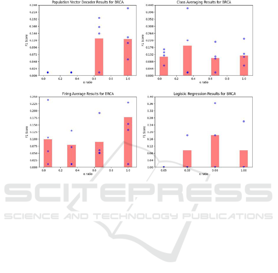
Figure 4: Results for different population decoding methods of SNNs trained on datasets with varying levels of synthetic

oversampling. Each red bar represents the score over the entire dataset, whereas each blue dot represents the score for a single

fold.

this is due to every neuron in the output population

being associated with the majority class, thereby

rendering the system unable to make predictions of

the minority class. Logistic regression had similar

issues with performance on the default dataset with a

low α ratio, but saw a marked improvement at the

point of oversampling to α=0.33 for BRCA and

α=0.66 for KIRC, and performed reasonably well

above these thresholds. Class averaging and firing

averaging both performed considerably better across

all α values. They therefore demonstrate resilience to

class imbalance, as there appears to be no strong

correlation between their predictive performance and

α ratio. Across both datasets, class averaging had

the highest single performance of any population

decoding method trialled in this research.

4.2 Distribution of Neuron Class

Assignments

Herein lies an exploration of neuron class

assignments. Presented in Figure 5 is a heatmap of the

α ratio of neuron class assignments determined via

Equation (2). We further calculate the Pearson

correlation coefficient between the α ratio of the

training dataset and the neuron class assignments:

The BRCA dataset has a dataset-neuron α correlation

coefficient of 0.932, and KIRC 0.879. Both datasets

showing such a strong correlation is certainly

indicative of the relationship between the distribution

of neuron classes and classes in the training set. This

result is notable as one may expect, for instance, that

the number of neurons assigned to a certain class be

dependent upon the complexity of the stimuli within

that class. Querlioz et al. (2013) ascribe the

improvement of predictive performance when

increasing the size of the population of output

neurons to the notion that the population is able to

learn more diverse representations of the output class.

However, as our chosen SMOTE technique is to

simply oversample the minority class, complexity of

the stimuli is constant across varying levels of α ratio.

From these results, we suggest that the determining

factor for the class assignment would therefore appear

to be the class distribution of the stimulus set. Another

point of interest is that whilst the correlation between

the α ratios is high, the heatmap in Figure 5 shows

that the relationship is not exactly linear. On the

unmodified datasets, the low α ratio leads to mode

collapse, where every neuron in the output population

Neural Population Decoding and Imbalanced Multi-Omic Datasets for Cancer Subtype Diagnosis

399

is assigned to the majority class. For the highest α

ratio, where the dataset was synthetically

oversampled to have an equal class distribution, the

neuron class distribution also reaches a similarly high

α ratio. However, for both the α=0.33 and α=0.66

datasets, there is a much larger discrepancy between

the dataset and neuron assignments. This is likely

indicative of the shortcomings of Equations (1) & (2)

when dealing with class imbalance which we

introduced in Section 2 – regardless of whether a

neuron is presented with 3 or 6 examples from the

minority class, if it’s shown 10 from the majority

class then it has a considerably greater likelihood of

being assigned as a majority neuron. This hypothesis

further explains the “jump” in neuron assignments

when moving from α=0.66 to α=1.0, as the minority

class is finally placed on equal footing with the

majority class.

Figure 5: Heatmap of the relationship between the α ratio

of neuron class assignments versus the class distribution of

the training set. The numerical value within each cell is the

α ratio of neuron assignments for each of the K-folds during

training. The colour scale represents the absolute difference

between the neuron assignment α ratio and the α ratio of

the training set.

4.3 Multi versus Single Omics

In this section, we analyse the network’s performance

when trained on subsets of the omic information

present in the BRCA dataset. The results of these

experiments are shown in Figure 6. Our results

generally concur with that of other researchers in

relation to the predictive power of the omic types

(Fatima & Rueda, 2020). Utilising all multi-omic

features together leads to the best classification

results. This is followed by genomic, mitochondrial

RNA, and methylation features (respectively). These

results are encouraging as they support the network’s

claim to be effectively learning information from the

input stimuli, despite the fact that the overall

classification is quite poor in comparison with other

techniques applied to TCGA datasets (Fatima &

Rueda, 2020).

4.4 Test Set Bias

Here, we demonstrate the effects of the bias

introduced by performing population decoding using

the responses to a test set, and then predicting on that

same test set. First, consider using a trained WTA

network to perform classification upon a test set,

using any of the population decoding methods

defined in Section 2 where Z is a prerequisite (i.e. not

logistic regression). In this example, we set the initial

size of the test set to only one stimulus sample.

Following Equation (1) to construct Z, we notice that

it is impossible for the system to produce an incorrect

prediction; whichever neuron(s) spiked when

presented with the stimulus are retroactively assigned

to be a neuron of that class. Shown in Figure 6 is the

accuracy score when using a completely untrained

network’s responses over various sized subsets of the

testing set to determine neuron class associations. We

use accuracy score in this case rather than F1, as the

randomly distributed test subsets may not contain any

positive samples, thereby making F1 inapplicable. We

can clearly see from Figure 7 that the “infallible

neuron” problem arises when the size of the test set

has a low number of samples. We can further

determine that the bias introduced by this

methodology decreases as the number of test samples

increases. This is likely why the issue was not

identified by Himst et al. (2023) & Guo et al. (2017)

when working with the 10,000 sample MNIST testing

set, but is certainly something to be wary of with

smaller datasets. We posit that this may also be a

contributing factor to the ability of these systems to

have such high performance whilst only being

exposed to the training set for one epoch, whereas

Nessler et al. (2013), Diehl & Cook (2015) and

Querlioz et al. (2013) all required multiple epochs to

achieve similar results. Luckily, the solution we

propose to address this bias is extremely simple: use

BIOINFORMATICS 2024 - 15th International Conference on Bioinformatics Models, Methods and Algorithms

400

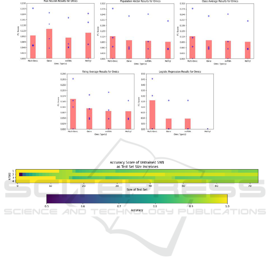
Figure 6: F1 score results for the WTA network trained on various subsets of omic information using K-folds cross validation.

Each bar represents the score over the entire dataset, whereas each blue dot represents the score for a single fold.

Figure 7: Heatmap of the accuracy score results of an untrained SNN making predictions upon a test set of increasing size,

where the population decoding is calculated using the responses of the network to that same test. The results shown here are

calculated over the BIRC dataset split into 4 folds.

the network responses from the training set to

perform population decoding, rather than the test set

responses. This removes the need to use test labels to

make predictions, and importantly eliminates the

infallible neuron problem. One additional piece of

advice for practitioners making this change is to only

start record training responses after the network has

been trained for a desired number of epochs, as using

the responses from an untrained network is liable to

give poor results. Diehl & Cook (2015) show that

following these practices can still lead to strong

classification performance.

5 CONCLUSION

Throughout this work, we have explored the

motivation and implications of implementing an array

of both common and novel population decoding

strategies for multi-omic based cancer subtype

diagnosis. Our findings show that the winner-take-all

and population vector decoders are both heavily

impacted by class imbalance, whereas class

averaging, logistic regression, and our novel firing

average implementation are more imbalance

resistant. We further show that the assignment of

neuron classes in population decoders is highly

correlated with the class distribution of the stimulus

set. This is a property which has, as far as we can

identify, gone unnoted thus far in the literature, and

warrants further investigation into the relationship

between the complexity of stimuli, class distribution

and neuron assignments.

Overall, the predictive performance of our system

is poor in comparison to other methods using this

dataset (Fatima & Rueda, 2020). In our estimation,

the primary issue lies in the loss of information when

transforming multi-omic data into binarized GSN

Neural Population Decoding and Imbalanced Multi-Omic Datasets for Cancer Subtype Diagnosis

401

images. We can observe from Figure 1 that a simple

logistic regression model is capable of achieving

near-perfect results using the same feature subset,

thereby isolating the problem to either the GSN or the

SNN. We later tested the classification performance

of a simple Convolutional Neural Network (CNN) on

the GSN images, which likewise had difficulty

extracting information from the binary data, and

surprisingly lead to even poorer predictive

performance than the SNN system. Thus, we

conclude that more sophisticated methods of

information encoding are necessary if we wish to

apply SNNs to datasets of within the domain of multi-

omics, or indeed to continuous tabular datasets in

general.

Despite the quality of our predictions, we are

nevertheless able to identify issues with current

practices in regards to the bias introduced by utilising

testing set labels and responses to perform population

decoding. Our recommendation for future researchers

is that this practice be avoided in favour of using the

training set, with the caveat that the network be

trained for at least one epoch before collecting the

responses.

Several challenges that we faced during this

research were related to the highly stochastic nature

of Bayesian WTA networks. This leads to high

variance in training convergence, making the

system’s performance difficult to evaluate in general

terms. K-folds cross validation is absolutely

necessary in this instance to gain insight into the

variance of results between runs. Furthermore, due to

their non-parallelizable nature and high

dimensionality requirements, training times can be

exceedingly long (Querlioz et al. (2013) report

approximately 8 hours for one run on the MNIST

dataset). Combined, these two factors make iterative

improvement difficult, as well as making it intractable

to explore high dimensional hyperparameter spaces.

One area for future research could therefore be the

application of more computing power to properly

perform hyperparameter optimisation on the network,

which could lead to superior performance.

Future research may alternatively wish to focus on

a biologically plausible method of translating

population responses into discrete decisions. One

potential direction for this is suggested by Hao et al.

(2020), wherein they combine the unsupervised

STDP learning rule with a leaky integrate-and-fire

neuron model to perform classification on the MNSIT

dataset. We have identified the encoding of

information as a bottleneck, as SNNs necessitate the

discretisation of information into spikes, inherently

impairing the maximum information density of the

system. To perhaps alleviate this problem, further

research could attempt alternative spike encoding

methods, such as those suggested by Guo et al.

(2021). On the other end of the system, interesting

insights could be gained by investigating the temporal

nature of neural responses, as opposed to the spike

count code (Grün & Rotter, 2010).

REFERENCES

Yamazaki K, Vo-Ho VK, Bulsara D, Le N. Spiking Neural

Networks and Their Applications: A Review. Brain Sci.

2022 Jun 30;12(7):863.

van der Himst, O., Bagheriye, L., & Kwisthout, J. (2023,

August). Bayesian Integration of Information Using

Top-Down Modulated WTA Networks. arXiv e-prints,

arXiv:2308.15390. doi: 10.48550/arXiv.2308.15390

Ma WJ, Pouget A. Population codes: Theoretic aspects.

Encyclopedia of neuroscience. 2009 Jun;7:749-55.

Guo, S., Yu, Z., Deng, F., Hu, X., & Chen, F. (2017).

Hierarchical bayesian inference and learning in

spiking neural networks. IEEE transactions on

cybernetics, 49 (1), 133–145.

Grün, S. and Rotter, S. eds., 2010. Analysis of parallel spike

trains (Vol. 7). Springer Science & Business Media.

J. M. Beck et al., Probabilistic population codes for

Bayesian decision making, Neuron, vol. 60, no. 6, pp.

1142–1152, 2008.

Shamir, M. (2009, 02). The temporal winner-take-all

readout. PLOS Computational Biology, 5 (2), 1-13.

doi:10.1371/journal.pcbi.1000286.

D. Kersten, P. Mamassian, and A. Yuille, Object perception

as bayesian inference, Annual Review of Psychology,

vol. 55, no. 1, pp. 271–304, 2004, pMID: 14744217.

T. S. Lee and D. Mumford, Hierarchical Bayesian inference

in the visual cortex, J. Opt. Soc. America A Opt. Image

Sci. Vis., vol. 20, pp. 1434–1448, 2003.

K. Friston, The free-energy principle: A unified brain

theory?, Nat. Rev. Neurosci., vol. 11. 127–138, 2010.

B. Nessler, M. Pfeiffer, L. Buesing, W. Maass, Bayesian

computation emerges in generic cortical microcircuits

through spiketiming-dependent plasticity, PLoS

Comput. Biol., vol. 9, no. 4, 2013, Art. no. e1003037.

P. U. Diehl and M. Cook, Unsupervised learning of digit

recognition using spike-timing-dependent plasticity,

Front. Comput. Neurosci., vol. 9, p. 99, Aug. 2015

Querlioz, Damien & Bichler, Olivier & Dollfus, Philippe &

Gamrat, Christian. (2013). Immunity to Device

Variations in a Spiking Neural Network With

Memristive Nanodevices. IEEE Transactions on

Nanotechnology. 12. 288-295.

10.1109/TNANO.2013.2250995.

Hao, Y., Huang, X., Dong, M., & Xu, B. (2020). A

biologically plausible supervised learning method for

spiking neural networks using the symmetric stdp rule.

Neural Networks, 121, 387-395 doi:

https://doi.org/10.1016/j.neunet.2019.09.007.

BIOINFORMATICS 2024 - 15th International Conference on Bioinformatics Models, Methods and Algorithms

402

Weinstein, J.N.Collisson, E. A. Mills, G. B.Shaw, K.R.

Ozenberger, B.A.Stuart (2013, October). The cancer

genome atlas pan-cancer analysis project, Cancer

Genome Atlas Research Network, Nat Genet, 45 (10),

1113-1120.

Fatima, N., & Rueda, L. (2020, 05). iSOM-GSN: an

integrative approach for transforming multi-omic data

into gene similarity networks via self-organizing maps.

Bioinformatics, 36 (15), 4248-4254.

Ang, JC & Mirzal, Andri & Haron, Habibollah & Hamed,

Haza Nuzly Abdull. (2015). Supervised, Unsupervised,

and Semi-Supervised Feature Selection: A Review on

Gene Selection. IEEE/ACM Transactions on

Computational Biology and Bioinformatics. 13.

Ding C, Peng H. Minimum redundancy feature selection

from microarray gene expression data. J Bioinform

Comput Biol. 2005;3(2):185-205.

T. Kohonen, The self-organizing map, in Proceedings of the

IEEE, vol. 78, no. 9, pp. 1464-1480, Sept. 1990, doi:

10.1109/5.58325.

Guo, Wenzhe & Fouda, Mohammed E. & Eltawil, Ahmed

& Salama, Khaled. (2021). Neural Coding in Spiking

Neural Networks: A Comparative Study for Robust

Neuromorphic Systems. Frontiers in Neuroscience. 15.

638474. 10.3389/fnins.2021.638474.

Chawla, Nitesh & Bowyer, Kevin & Hall, Lawrence &

Kegelmeyer, W. (2002). SMOTE: Synthetic Minority

Over-sampling Technique. J. Artif. Intell. Res. (JAIR).

16. 321-357. 10.1613/jair.953.

Imbalanced-learn: SMOTE. (2016). Imbalanced-learn.

Retrieved September 30, 2023.

Neural Population Decoding and Imbalanced Multi-Omic Datasets for Cancer Subtype Diagnosis

403