Integrating Structure and Sequence: Protein Graph Embeddings via

GNNs and LLMs

Francesco Ceccarelli

, Lorenzo Giusti

, Sean B. Holden

and Pietro Li

Department of Computer Science and Technology , University of Cambridge, Cambridge, U.K.

Department of Computer, Control and Management Engineering, Sapienza University, Rome, Italy

Keywords:

Graph Neural Networks, Large Language Models, Protein Representation Learning.

Abstract:

Proteins perform much of the work in living organisms, and consequently the development of efﬁcient com-

putational methods for protein representation is essential for advancing large-scale biological research. Most

current approaches struggle to efﬁciently integrate the wealth of information contained in the protein sequence

and structure. In this paper, we propose a novel framework for embedding protein graphs in geometric vector

spaces, by learning an encoder function that preserves the structural distance between protein graphs. Utiliz-

ing Graph Neural Networks (GNNs) and Large Language Models (LLMs), the proposed framework generates

structure- and sequence-aware protein representations. We demonstrate that our embeddings are successful

in the task of comparing protein structures, while providing a signiﬁcant speed-up compared to traditional

approaches based on structural alignment. Our framework achieves remarkable results in the task of protein

structure classiﬁcation; in particular, when compared to other work, the proposed method shows an average

F1-Score improvement of 26% on out-of-distribution (OOD) samples and of 32% when tested on samples

coming from the same distribution as the training data. Our approach ﬁnds applications in areas such as drug

prioritization, drug re-purposing, disease sub-type analysis and elsewhere.

1 INTRODUCTION

Proteins are organic macro-molecules made up of

twenty types of natural amino acids. Almost all in-

teractions and reactions which occur in living organ-

isms, from signal transduction, gene transcription and

immune function to catalysis of chemical reactions,

involve proteins (Morris et al., 2022). The compari-

son of proteins and their structures is an essential task

in bioinformatics, providing support for protein struc-

ture prediction (Kryshtafovych et al., 2019), the study

of protein-protein docking (Lensink et al., 2018),

structure-based protein function prediction (Gherar-

dini and Helmer-Citterich, 2008) and many further

tasks. Considering the large quantity of protein data

stored in the Protein Data Bank (PDB) (Berman et al.,

2003) and the rapid development of methods for per-

forming protein structure prediction (for example, Al-

phaFold2 (Jumper et al., 2021)), it is desirable to de-

velop methods capable of efﬁciently comparing the

tertiary structures of proteins.

Generally, protein comparison methods can be

divided into two classes: alignment-based meth-

ods (Akdel et al., 2020; Shindyalov and Bourne,

1998; Kihara and Skolnick, 2003) and alignment-free

methods (Xia et al., 2022; Røgen and Fain, 2003;

Budowski-Tal et al., 2010; Zotenko et al., 2006). The

former aim at ﬁnding the optimal structural super-

position of two proteins. A scoring function is then

used to measure the distance between each pair of

superimposed residues. For such methods (for ex-

ample (Holm and Sander, 1993; Zhang and Skol-

nick, 2005)) the superposition of the atomic structures

is the main bottleneck as it has been proven to be

an NP-hard problem (Lathrop, 1994). On the other

hand, alignment-free methods try to represent each

protein in the form of a descriptor, and then to mea-

sure the distance between pairs of descriptors (Xia

et al., 2022). Descriptors need to satisfy two require-

ments: (1) their size should be ﬁxed and independent

of the length of proteins; (2) they should be invariant

to rotation and translation of proteins.

The template modeling score (TM-score) (Zhang

and Skolnick, 2004) is a widely used metric for as-

sessing the structural similarity between two pro-

teins. It is based on the root-mean-square deviation

(RMSD) of the atomic positions in the proteins, but

considers the lengths of the proteins and the number

582

Ceccarelli, F., Giusti, L., Holden, S. and Liò, P.

Integrating Structure and Sequence: Protein Graph Embeddings via GNNs and LLMs.

DOI: 10.5220/0012453600003654

Paper published under CC license (CC BY-NC-ND 4.0)

In Proceedings of the 13th International Conference on Pattern Recognition Applications and Methods (ICPRAM 2024), pages 582-593

ISBN: 978-989-758-684-2; ISSN: 2184-4313

of residues that can be superimposed. TM-score has

been shown to be highly correlated with the similar-

ity of protein structures and can be used to identify

structurally similar proteins, even when they have low

sequence similarity. Unfortunately, computing TM-

scores is computationally intractable even for rela-

tively small numbers of proteins. TM-align (Zhang

and Skolnick, 2005), one of the popular alignment-

based methods, takes about 0.5 seconds for one struc-

tural alignment on a 1.26 GHz PIII processor. As

such, computing TM-scores for existing databases,

containing data for millions of proteins, is unafford-

able. While several deep learning methods for protein

comparison have been developed (for example, Deep-

Fold (Liu et al., 2018) and GraSR (Xia et al., 2022))

they suffer from major drawbacks: (1) they are trained

by framing the protein comparison task as a classi-

ﬁcation problem—that is, predicting if two proteins

are structurally similar—and hence fail to directly in-

corporate TM-scores in the loss function formulation;

(2) they produce latent representations (embeddings)

which do not integrate the information contained in

the protein sequences and structures; (3) they usually

do not exploit the inductive bias induced by the topol-

ogy of graph-structured proteins, and they fail to con-

sider different geometries of the latent space to match

well the underlying data distribution.

In this paper, we address the aforementioned lim-

itations of current protein embedding methods by

proposing an efﬁcient and accurate technique that in-

tegrates both protein sequence and structure infor-

mation. In detail, we ﬁrst construct protein graphs

where each node represents an amino acid in the pro-

tein sequence. We then generate features for each

amino acid (node in the graph) using Large Language

Models (LLMs) before applying Graph Neural Net-

works (GNNs) to embed the protein graphs in geo-

metric vector spaces while combining structural and

sequence information. By incorporating TM-scores

in the formulation of the loss function, the trained

graph models are able to learn a mapping that pre-

serves the distance between the input protein graphs,

providing a way to quickly compute similarities for

every pair of unseen proteins. We evaluated the pro-

posed approach and its ability to generate meaning-

ful embeddings for downstream tasks on two protein

datasets. On both, the proposed approach reached

good results, outperforming other current state-of-

the-art methods on the task of structural classiﬁcation

of proteins on the SCOPe dataset (Fox et al., 2014).

Contribution. The main contributions of this paper

can be summarised as follow: (i) A novel learning

framework for generating protein representations in

geometric vector spaces by merging structural and se-

quence information using GNNs and LLMs. (ii) A

quick and efﬁcient method for similarity computation

between any pair of proteins. (iii) An evaluation of

the ability of our embeddings, in both supervised and

unsupervised settings, to solve downstream protein

classiﬁcation tasks, and a demonstration of their su-

perior performance when compared to current state-

of-the-art methods. Our approach ﬁnds a plethora of

applications in the ﬁelds of bioinformatics and drug

discovery.

2 BACKGROUND AND RELATED

WORK

Several alignment-based methods have been proposed

over the years, each exploiting different heuristics to

speed up the alignment process. For example, in

DALI (Holm and Sander, 1999), Monte Carlo opti-

mization is used to search for the best structural align-

ment. In Shindyalov and Bourne (1998), the authors

proposed combinatorial extension (CE) for similarity

evaluation and path extension. An iterative heuristic

based on the Needleman–Wunsch dynamic program-

ming algorithm (Needleman and Wunsch, 1970) is

employed in TM-align (Zhang and Skolnick, 2005),

SAL (Krishna et al., 1997) and STRUCTAL (Zhang

and DeLisi, 1997). Examples of alignment-free ap-

proaches are Scaled Gauss Metric (SGM) (Røgen

and Fain, 2003) and the Secondary Structure Element

Footprint (SSEF) (Zotenko et al., 2006). SGM treats

the protein backbone as a space curve to construct a

geometric measure of the conformation of a protein,

and then uses this measure to provide a distance be-

tween protein shapes. SSEF splits the protein into

short consecutive fragments and then uses these frag-

ments to produce a vector representation of the pro-

tein structure as a whole. More recently, methods

based on deep learning have been developed for the

task of protein structure comparison. For instance,

DeepFold (Liu et al., 2018) used a deep convolu-

tional neural network model trained with the max-

margin ranking loss function (Wang et al., 2016) to

extract structural motif features of a protein, and learn

a ﬁngerprint representation for each protein. Cosine

similarity was then used to measure the similiarity

scores between proteins. DeepFold has a large num-

ber of parameters, and fails to exploit the sequence in-

formation and the topology of graph-structured data.

GraSR (Xia et al., 2022) employs a contrastive learn-

ing framework, GNNs and a raw node feature extrac-

tion method to perform protein comparison. Com-

pared to GraSR, we present a general framework to

produce representations of protein graphs where the

Integrating Structure and Sequence: Protein Graph Embeddings via GNNs and LLMs

583

distance in the embedding space is correlated with the

structural distance measured by TM-scores between

graphs. Finally, our approach extends the work pre-

sented in Corso et al. (2021), which was limited to bi-

ological sequence embeddings, to the realm of graph-

structured data.

3 MATERIAL AND METHODS

The core approach, shown in Figure 1, is to map

graphs into a continuous space so that the distance be-

tween embedded points reﬂects the distance between

the original graphs measured by the TM-scores. The

main components of the proposed framework are the

geometry of the latent space, a graph encoder model,

a sequence encoder model, and a loss function. De-

tails for each are as follows.

3.1 Latent Space Geometry

The distance function used (d in Figure 1) deﬁnes the

geometry of the latent space into which embeddings

are projected. In this work we provide a comparison

between Euclidean, Manhattan, Cosine and squared

Euclidean (referred to as Square) distances (details in

Appendix B).

3.2 Graph Encoder Model

The encoder performs the task of mapping the in-

put graphs to the embedding space. A variety of

models exist for this task, including linear, Multi-

layer Perceptron (MLP), LSTM (Cho et al., 2014),

CNN (Fukushima, 1980) and Transformers (Vaswani

et al., 2017). Given the natural representation of pro-

teins as graphs, we chose GNNs as encoder mod-

els. We have constructed the molecular graphs of

proteins starting from PDB ﬁles. A PDB ﬁle con-

tains structural information such as 3D atomic coor-

dinates. Let G = (V, E) be a graph representing a pro-

tein, where each node v ∈ V is a residue and inter-

action between the residues is described by an edge

e ∈ E. Two residues are connected if they have any

pair of atoms (one from each residue) separated by

a Euclidean distance less than a threshold distance.

The typical cut-off, which we adopt in this work, is 6

angstroms (

A) (Chen et al., 2021).

3.3 Sequence Encoder Model

Given the graph representation of a protein, each

node v of the graph (each residue) must be associ-

ated with a feature vector. Typically, features ex-

Table 1: Investigated node attributes and their dimensions.

BERT and LSTM features are extracted using LLMs pre-

trained on protein sequences (ProBert (Brandes et al., 2022)

and SeqVec (Heinzinger et al., 2019)).

Feature Dimension

One hot encoding of amino acids 20

Physicochemical properties 7

BLOcks SUbstitution Matrix 25

BERT-based language model 1024

LSTM-based language model 1024

tracted from protein sequences by means of LLMs

have exhibited superior performances compared to

handcrafted features. We experimented with ﬁve dif-

ferent sequence encoding methods: (1) a simple one-

hot encoding of each residue in the graph, (2) seven

physicochemical properties of residues as extracted

by Meiler et al. (2001), which are assumed to in-

ﬂuence the interactions between proteins by creat-

ing hydrophobic forces or hydrogen bonds between

them, (3) the BLOcks SUbstitution Matrix (BLO-

SUM) (Henikoff and Henikoff, 1992), which counts

the relative frequencies of amino acids and their sub-

stitution probabilities, (4) features extracted from pro-

tein sequences employing a pre-trained BERT-based

transformer model (ProBert (Brandes et al., 2022)),

and (5) node features extracted using a pre-trained

LSTM-based language model (SeqVec (Heinzinger

et al., 2019)). Table 1 summarizes the node features

and their dimensions, while Figure 2 depicts the pro-

cess of constructing a protein graph with node fea-

tures, starting from the corresponding protein data.

3.4 Loss Function

The loss function used, which minimises the MSE be-

tween the graph distance and its approximation as the

distance between the embeddings, is

L =

∑

∈G

(TM(g

, g

) −d (GNN

), GNN

)))

(1)

where G is the training set of protein graphs,

GNN

is the graph encoder and θ represents the pa-

rameters of the model. The TM-score is a similarity

metric in the range (0,1], where 1 indicates a perfect

match between two structures. Since the formulation

of the loss is expressed in terms of distances, we re-

formulate the TM-scores as a distance metric by sim-

ply computing TM(g

, g

) = 1 − TM

score

, g

). By

training neural networks to minimize the loss in Equa-

tion 1, we encourage the networks to produce latent

representations such that the distance between these

representations is proportional to the structural dis-

tance between the input graphs.

ICPRAM 2024 - 13th International Conference on Pattern Recognition Applications and Methods

584

Structural !

Distance

Input proteins Protein Graphs with sequence attributes

Graph Encoder

3-Dimensional Latent Space

of Protein Graphs

Structural comparison

Protein structural

classiﬁcation

Protein function

prediction

Example applications of protein

embeddings

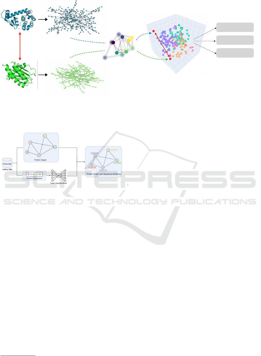
Figure 1: We learn an encoder function that preserves the structural distance, measured by the TM-score, between two input

proteins. We construct protein graphs by combining sequence and structure information as shown in Figure 2. A distance

function d deﬁnes the shape of the latent space. The generated embeddings can be used for a variety of applications in

bioinformatics and drug discovery. (For simplicity, this Figure depicts a 3-dimensional latent space.).

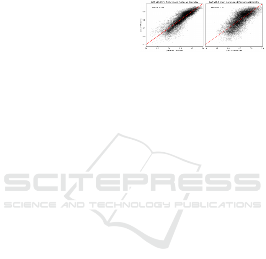
Figure 2: Graph representation of a protein, which com-

bines sequence and structure. Starting from protein data (a

PDB ﬁle from, for example, UniProt or PDB), we extract

protein sequence and structure information. We construct

graphs where each node represents an amino acid in the pro-

tein sequence. We then generate features for each node in

the graph using Large Language Models pre-trained on pro-

tein sequences.

4 PROTEIN DATASETS

We evaluated the proposed approach on two pro-

tein datasets. First, we downloaded the human pro-

teome from UniProt

and sub-selected 512 protein

kinases. To obtain the TM-scores to train the graph

models, we evaluated the structural similarity using

TM-align (Zhang and Skolnick, 2005). All-against-

all alignment yielded a dataset composed of 130,816

total comparisons. Every kinase in the dataset is cat-

egorized in one of seven family groups: (a) AGC

(63 proteins), (b) CAMK (82 proteins), (c) CK1 (12

proteins), (d) CMGC (63 proteins), (e) STE (48 pro-

teins), (f) TK (94 proteins), and (g) TKL (43 pro-

teins). The number of nodes in the graphs ranges from

https://www.uniprot.org

253 to 2644, with an average size of approximately

780 nodes. The average degree in the graphs is ap-

proximately 204, the average diameter of the graphs

is approximately 53 nodes and the maximum diam-

eter is 227 nodes. We further used the 40% iden-

tity ﬁltered subset of SCOPe v2.07 (March 2018) as

a benchmark dataset (Fox et al., 2014). This dataset

contains 13,265 protein domains classiﬁed in one of

seven classes: (a) all alpha proteins (2286 domains),

(b) all beta proteins (2757 domains), (c) alpha and

beta proteins (a/b) (4148 domains), (d) alpha and beta

proteins (a+b) (3378 domains), (e) multi-domain pro-

teins (alpha and beta) (279 domains), (f) membrane

and cell surface proteins and peptides (213 domains),

and g) small proteins (204 domains). We again used

TM-align with all-against-all settings to construct a

dataset of approximately 170 millions comparisons.

To reduce the computational time and cost during

training, we randomly sub-sampled 100 comparisons

for each protein to create a ﬁnal dataset of 1,326,500

comparisons. For this dataset, the number of nodes

in the graphs ranges from 30 to 9800, with an aver-

age size of approximately 1978 nodes. The average

degree is approximately 90, the average diameter of

the graphs is approximately 9 nodes and the maxi-

mum diameter is 53 nodes. Compared to benchmark

graph datasets (for example Sterling and Irwin (2015)

and Dwivedi et al. (2022)) we evaluated our approach

on graphs of signiﬁcantly larger size (84 and 13 times

more nodes than the molecular graphs in Sterling and

Irwin (2015) and in Dwivedi et al. (2022), respec-

tively).

Integrating Structure and Sequence: Protein Graph Embeddings via GNNs and LLMs

585

5 EXPERIMENTAL RESULTS

5.1 Experimental Settings

We evaluate the proposed framework using Graph

Convolutional Networks (GCNs) (Kipf and Welling,

2016), Graph Attention Networks (GATs) (Veli

ckovi

et al., 2017), and GraphSAGE (Hamilton et al., 2017)

(Appendix A). All the models were implemented

with two graph layers in PyTorch geometric (Fey and

Lenssen, 2019) to learn protein embeddings of size

256. Adam optimizer (Kingma and Ba, 2014) with

a learning rate of 0.001 was used to train the mod-

els for 100 epochs with a patience of 10 epochs. The

batch size was set to 100. We used 4 attention heads

in the GAT architecture. For each model, Rectiﬁed

Linear Units (ReLUs) (Nair and Hinton, 2010) and

Dropout (Srivastava et al., 2014) were applied after

each layer, and mean pooling was employed as read-

out function to obtain graph-level embeddings from

the learned node-level representations. Finally, each

experiment was run with 3 different seeds to provide

uncertainty estimates.

5.2 Kinase Embeddings

For the generation of the embeddings, we used 80%

of the kinase proteins for training and the remaining

20% for testing. Table 2

shows the MSE values for the graph encoders, us-

ing different choices of distance functions and node

features. For each model, the best scores are con-

sistently reached with LSTM-extracted features and

Euclidean geometry of the embedding space. Across

all models, GAT embeddings exhibit the lowest MSE,

followed by GarphSAGE and GCN. From Table 2, it

is clear that using pre-trained language models to ex-

tract node features from protein sequences leads to

better results. MSE scores for all distances across

all encoder models are lower when using BERT and

LSTM features. Furthermore, the LSTM-extracted

features perform consistently better compared to the

BERT ones. BLOSUM and Physicochemical features

are also usually associated with higher MSE for all

distances and models, indicating that they are poorly

correlated to TM-scores.

5.3 Fast Inference of TM-Scores

We employed the trained GAT architectures from Ta-

ble 2 to predict the TM-scores for the kinase pairs in

the test set. In Figure 3, we show the predicted versus

actual TM-scores for two combinations of features

and embedding geometries. The left plot in Figure 3

Figure 3: Actual versus predicted TM-scores. Using LSTM

features and Euclidean geometry (left) results in predictions

which follow more tightly the red line of the oracle com-

pared to BLOSUM features in the Manhattan space (right).

uses LSTM-extracted features and Euclidean space,

while the right one shows predictions for BLOSUM

features and Manhattan space. The complete quan-

titative evaluations, measured by Pearson correlation

between model predictions and true TM-scores for all

distances and features, are reported in Appendix D.

As in Table 2, the best performances are reached when

employing LSTM and BERT features while BLO-

SUM and Physicochemical features lead to the poor-

est performances (Appendix D). The highest correla-

tion score, reﬂecting the results reported in Table 2,

is reached when employing LSTM features and Eu-

clidean distance (Figure 3). It is worth noticing that,

for the 26,164 comparisons in the test set, the pro-

posed approach took roughly 120 seconds to compute

TM-scores. Executing TM-align with the same num-

ber of comparisons took 57,659 seconds (≈ 16 hours).

Details of the TM-score inference times for all the

models are given in Appendix D. The major speed-

up provided by performing inference using machine

learning models makes the proposed approach appli-

cable to datasets comprising millions of proteins.

5.4 Ablation Study: Structure Removal

Coupling GNNs with LLMs provides a means of in-

tegrating the information coming from the structure

and sequence of proteins. To analyse the beneﬁts of

exploiting the topology induced by the graph struc-

tures, we performed an ablation study which disre-

gards such information. DeepSet (Zaheer et al., 2017)

considers objective functions deﬁned on sets, that are

invariant to permutations. Using a DeepSet formu-

lation, we constructed protein graphs with features

where each node is only connected to itself. As for

the graph models, we trained DeepSet to minimize

the loss function in Equation 1 and report the results

in Table 3. Similarly to Table 2, the best MSE scores

are reached when using LSTM features and Euclidean

geometry. The scores in Table 3, computed by disre-

garding the graph connectivity and neighborhood in-

formation, are signiﬁcantly higher than those reported

ICPRAM 2024 - 13th International Conference on Pattern Recognition Applications and Methods

586

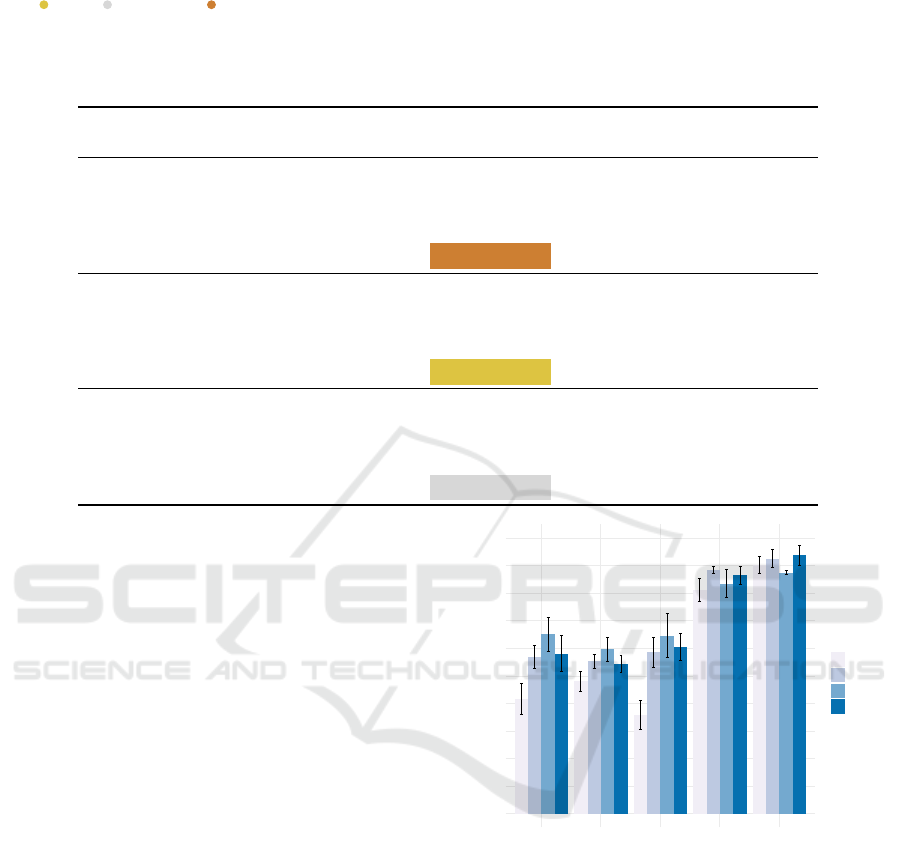
Table 2: MSE results for different feature types, distance functions and graph encoder models on the kinase dataset. We use

gold , silver , and bronze colors to indicate the ﬁrst, second and third best performances, respectively. For each model,

the best scores are consistently reached with LSTM-extracted features and Euclidean geometry of the embedding space.

Across all models, GAT embeddings exhibit the best performance. For all the models, MSE scores are lower for features

extracted by means of LLMs (BERT and LSTM) compared to handcrafted feature extraction methods (one-hot, biochemical

and BLOSUM).

Model Feature Distance

Cosine Euclidean Manhattan Square

GCN

One hot 0.0194 ± 0.002 0.0380 ± 0.003 0.0192 ± 0.001 0.0729 ± 0.004

Physicochemical 0.0343 ± 0.012 0.0483 ± 0.009 0.0397 ±0.003 0.1109 ±0.007

BLOSUM 0.0327 ± 0.071 0.0271 ±0.043 0.0450±0.013 0.0697±0.023

BERT 0.0110 ± 0.003 0.0103 ± 0.001 0.0131 ± 0.006 0.0138 ±0.009

LSTM 0.0105 ±0.002 0.0088±0.004 0.0156 ± 0.001 0.0107 ± 0.004

GAT

One hot 0.0171 ± 0.001 0.0320 ± 0.012 0.0171 ± 0.011 0.0758 ± 0.009

Physicochemical 0.0295 ± 0.007 0.0328 ± 0.006 0.0220 ± 0.004 0.0856 ± 0.023

BLOSUM 0.0245 ± 0.012 0.0163 ± 0.009 0.0124 ± 0.011 0.0307 ± 0.009

BERT 0.0091 ± 0.018 0.0095 ± 0.008 0.0078 ± 0.009 0.0133 ± 0.011

LSTM 0.0088 ± 0.009 0.0073 ± 0.004 0.0086 ± 0.006 0.0101 ± 0.009

Graph

SAGE

One hot 0.0243 ± 0.002 0.0227 ± 0.011 0.0156 ± 0.009 0.0424 ± 0.010

Physicochemical 0.0301 ± 0.004 0.0266 ± 0.008 0.0310 ± 0.011 0.0578 ± 0.009

BLOSUM 0.0285 ± 0.007 0.0172 ± 0.008 0.0342 ± 0.002 0.0368 ± 0.007

BERT 0.0097 ± 0.011 0.0089 ± 0.007 0.0101 ± 0.007 0.0107 ± 0.009

LSTM 0.0093 ± 0.003 0.0084 ± 0.005 0.0143 ± 0.007 0.0094 ± 0.008

in Table 2 (p-value of t-test < 0.05 compared to GCN,

GAT and GraphSAGE). By considering patterns of

local connectivity and structural topology, GNNs are

able to learn better protein graph representations com-

pared to models which only exploit sequence-derived

features.

5.5 Downstream Task of Kinase

Classiﬁcation

To prove the usefulness of the learned embeddings for

downstream tasks, we set out to classify each kinase

into one of the seven family groups (AGC, CAMK,

CK1, CMGC, STE, TK, TKL). Using the embeddings

generated by the GAT models, we trained an MLP,

composed of 3 layers of size 128, 64 and 32 respec-

tively, and a SoftMax classiﬁcation head. The accu-

racy of classiﬁcation, computed as the average result

of 5-fold cross-validation, for each feature type and

distance function is reported in Figure 4. The results

are consistent with Table 2: the best accuracies are

obtained when using LSTM- and BERT-extracted se-

quence features, while handcrafted feature extraction

methods (one hot, BLOSUM and physicochemical)

provide the poorest performance. The highest accu-

racy values of 93.7% and 92.48% are reached with

LSTM features and Square and Euclidean distance

functions, respectively.

0.0

0.2

0.4

0.6

0.8

1.0

One Hot Physicochemical Blosum BERT LSTM

Feature

Accuracy

Distance

Cosine

Euclidean

Manhattan

Square

Figure 4: Accuracy of classiﬁcation for kinase family pre-

diction using the embeddings generated by the GAT models.

The highest accuracy value of 93.7% is reached with LSTM

features and the Square distance function.

5.6 Embedding out of Distribution

Samples

Being able to use pre-trained models for related or

similar tasks is essential in machine learning. We

tested the ability of the proposed graph models to

generalize to new tasks by generating embeddings for

the 13,265 proteins in the SCOPe dataset after being

trained only on kinase proteins. Given the better per-

formance provided by the use of LSTM features, in

this section we constructed protein graphs with LSTM

Integrating Structure and Sequence: Protein Graph Embeddings via GNNs and LLMs

587

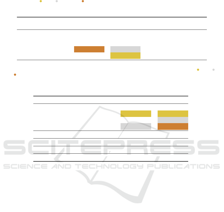
Table 3: MSE values for an ablation study which disregards the topological information induced by the structure of the protein

graphs. We use gold , silver , and bronze colors to indicate the ﬁrst, second and third best performances, respectively.

By ignoring the neighborhood and the structural information, the MSEs are signiﬁcantly higher (p-value of t-test < 0.05)

compared to GNNs.

Model Feature Distance

Cosine Euclidean Manhattan Square

DeepSet

One Hot 0.1742 ± 0.003 0.0421 ± 0.002 0.0358 ± 0.001 0.0714 ± 0.003

Physicochemical 0.1766 ± 0.010 0.0437 ± 0.006 0.0464 ± 0.004 0.0900 ± 0.006

BLOSUM 0.1553 ± 0.003 0.0381 ± 0.009 0.0558 ± 0.008 0.0914 ± 0.008

BERT features 0.0132 ± 0.004 0.0129 ± 0.005 0.0192 ± 0.005 0.0220 ± 0.004

LSTM features 0.0141 ± 0.003 0.0116 ± 0.010 0.0348 ± 0.006 0.0200 ± 0.007

Table 4: Out of distribution (OOD) classiﬁcation results on SCOPe proteins (F1-Score (OOD)). We use gold , silver , and

bronze colors to indicate the ﬁrst, second and third best performances, respectively. Despite the different training data, the

GAT model with Euclidean and Square geometry outperforms all other approaches trained on SCOPe proteins. Classiﬁcation

results for embeddings generated after training on SCOPe proteins are also shown (F1-Score); in this case, the proposed

approach outperforms the others by a larger margin for all choices of latent geometries.

Model Distance F1-Score (OOD) F1-Score

GAT

Cosine 0.6906 ± 0.0044 0.8290 ± 0.008

Euclidean 0.8204 ± 0.006 0.8557 ± 0.002

Manhattan 0.7055 ± 0.006 0.8481 ± 0.007

Square 0.8185 ± 0.004 0.8406 ± 0.006

SGM (Røgen and Fain, 2003) - - 0.6289

SSEF (Zotenko et al., 2006) - - 0.4920

DeepFold (Liu et al., 2018) - - 0.7615

GraSR (Xia et al., 2022) - - 0.8124

attributes and used a 3-Layer MLP as before to as-

sign the GAT-generated protein embeddings from the

SCOPe dataset to the correct class. Results of this

evaluation, measured as average F1-score across 5

folds for each distance function, are shown in Table 4

(F1-Score out of distribution (OOD)).

Euclidean and Square geometry of the embed-

ding space exhibited the best classiﬁcation perfor-

mances. Despite being trained on OOD samples, the

proposed framework with Euclidean and Square ge-

ometry still managed to outperform the current state-

of-the-art results reported from models trained and

tested on SCOPe proteins, as shown in Table 4. The

superior performance, despite the different training

data, suggests the ability of the proposed approach to

learn meaningful protein representations by (1) merg-

ing structural and sequence information into a sin-

gle pipeline, and (2) capturing different and relevant

properties of the geometries of the latent space into

which embeddings are projected.

5.7 Protein Structural Classiﬁcation

We constructed protein graphs with LSTM features

and trained the proposed GAT architectures on the

SCOPe dataset. The resulting MSE scores are re-

ported in Appendix D. The lowest score was again

reached when using Euclidean geometry for the latent

space. Using this model, we projected the protein em-

beddings onto two dimensions using t-SNE (Van der

Maaten and Hinton, 2008) as shown in Figure 5.

The high-level structural classes as deﬁned in SCOPe

were captured by the proposed embeddings. While

not directly trained for this task, combining struc-

tural and sequence information allowed us to identify

small, local clusters representing the different protein

families in the SCOPe dataset. We employed super-

vised learning and trained a 3-layer MLP classiﬁer

to label each protein embedding in the correct fam-

ily. Results of this evaluation, measured as average

F1-score across 5 folds, are shown in Table 4 (F1-

Score). When directly trained on SCOPe proteins, the

proposed approach outperforms the others by a large

margin for all choices of geometries (Table 4).

ICPRAM 2024 - 13th International Conference on Pattern Recognition Applications and Methods

588

Figure 5: t-SNE visualization of the learned embeddings,

coloured by protein structural family. The proposed ap-

proach generates protein embeddings which recapitulate the

different families in the SCOPe dataset.

6 CONCLUSION

In this paper, we presented a novel framework for

generating both structure- and sequence-aware pro-

tein representations. We mapped protein graphs with

sequence attributes into geometric vector spaces, and

showed the importance of considering different ge-

ometries of the latent space to match the underly-

ing data distributions. We showed that the gener-

ated embeddings are successful in the task of pro-

tein structure comparison, while providing an accu-

rate and efﬁcient way to compute similarity scores

for large-scale datasets, compared to traditional ap-

proaches (Appendix D). The protein graph represen-

tations generated by our approach showed state-of-

the-art results for the task of protein structural clas-

siﬁcation on the SCOPe dataset. This work opens op-

portunities for future research, with potential for sig-

niﬁcant contributions to the ﬁelds of bioinformatics,

structural protein representation and drug discovery

(Appendix E).

ACKNOWLEDGMENTS

For the purpose of open access, the author has applied

a Creative Commons Attribution (CC BY) licence to

any Author Accepted Manuscript version arising from

this submission. The protein structures in Figure 1

were downloaded from UniProt

2 3

under the Creative

Commons Attribution 4.0 International (CC BY 4.0)

License

and used without modiﬁcations.

https://www.uniprot.org

https://www.uniprot.org/help/license

https://creativecommons.org/licenses/by/4.0/

REFERENCES

Akdel, M., Durairaj, J., de Ridder, D., and van Dijk, A. D.

(2020). Caretta–a multiple protein structure alignment

and feature extraction suite. Computational and struc-

tural biotechnology journal, 18:981–992.

Berman, H., Henrick, K., and Nakamura, H. (2003). An-

nouncing the worldwide protein data bank. Nature

Structural & Molecular Biology, 10(12):980–980.

Brandes, N., Ofer, D., Peleg, Y., Rappoport, N., and Linial,

M. (2022). ProteinBERT: a universal deep-learning

model of protein sequence and function. Bioinformat-

ics, 38(8):2102–2110.

Budowski-Tal, I., Nov, Y., and Kolodny, R. (2010). Frag-

Bag, an accurate representation of protein structure,

retrieves structural neighbors from the entire PDB

quickly and accurately. Proceedings of the National

Academy of Sciences, 107(8):3481–3486.

Chen, J., Zheng, S., Zhao, H., and Yang, Y. (2021).

Structure-aware protein solubility prediction from se-

quence through graph convolutional network and pre-

dicted contact map. Journal of cheminformatics,

13(1):1–10.

Cho, K., Van Merri

enboer, B., Gulcehre, C., Bahdanau, D.,

Bougares, F., Schwenk, H., and Bengio, Y. (2014).

Learning phrase representations using RNN encoder-

decoder for statistical machine translation. arXiv

preprint arXiv:1406.1078.

Corso, G., Ying, Z., P

andy, M., Veli

ckovi

c, P., Leskovec,

J., and Li

o, P. (2021). Neural distance embeddings for

biological sequences. Advances in Neural Information

Processing Systems, 34:18539–18551.

Dwivedi, V. P., Ramp

sek, L., Galkin, M., Parviz, A., Wolf,

G., Luu, A. T., and Beaini, D. (2022). Long range

graph benchmark. Advances in Neural Information

Processing Systems, 35:22326–22340.

Fey, M. and Lenssen, J. E. (2019). Fast Graph Represen-

tation Learning with PyTorch Geometric. In ICLR

Workshop on Representation Learning on Graphs and

Manifolds.

Fox, N. K., Brenner, S. E., and Chandonia, J.-M.

(2014). SCOPe: Structural Classiﬁcation of Pro-

teins—extended, integrating SCOP and ASTRAL

data and classiﬁcation of new structures. Nucleic acids

research, 42(D1):D304–D309.

Fukushima, K. (1980). Neocognitron: A self-organizing

neural network model for a mechanism of pattern

recognition unaffected by shift in position. Biologi-

cal cybernetics, 36(4):193–202.

Gherardini, P. F. and Helmer-Citterich, M. (2008).

Structure-based function prediction: approaches and

applications. Brieﬁngs in Functional Genomics and

Proteomics, 7(4):291–302.

Gilmer, J., Schoenholz, S. S., Riley, P. F., Vinyals, O., and

Dahl, G. E. (2017). Neural message passing for quan-

tum chemistry. In International conference on ma-

chine learning, pages 1263–1272. PMLR.

Hamilton, W., Ying, Z., and Leskovec, J. (2017). Inductive

representation learning on large graphs. Advances in

neural information processing systems, 30.

Integrating Structure and Sequence: Protein Graph Embeddings via GNNs and LLMs

589

Heinzinger, M., Elnaggar, A., Wang, Y., Dallago, C.,

Nechaev, D., Matthes, F., and Rost, B. (2019). Mod-

eling aspects of the language of life through transfer-

learning protein sequences. BMC bioinformatics,

20(1):1–17.

Henikoff, S. and Henikoff, J. G. (1992). Amino acid sub-

stitution matrices from protein blocks. Proceedings

of the National Academy of Sciences, 89(22):10915–

10919.

Holm, L. and Sander, C. (1993). Protein structure com-

parison by alignment of distance matrices. Journal of

molecular biology, 233(1):123–138.

Holm, L. and Sander, C. (1999). Using dali for structural

comparison of proteins. Current opinion in structural

biology, 9(3):408–415.

Hu, J. X., Thomas, C. E., and Brunak, S. (2016). Network

biology concepts in complex disease comorbidities.

Nature Reviews Genetics, 17(10):615–629.

Jumper, J., Evans, R., Pritzel, A., Green, T., Figurnov,

M., Ronneberger, O., Tunyasuvunakool, K., Bates, R.,

ıdek, A., Potapenko, A., et al. (2021). Highly accu-

rate protein structure prediction with AlphaFold. Na-

ture, 596(7873):583–589.

Kihara, D. and Skolnick, J. (2003). The PDB is a covering

set of small protein structures. Journal of molecular

biology, 334(4):793–802.

Kingma, D. P. and Ba, J. (2014). Adam: A

method for stochastic optimization. arXiv preprint

arXiv:1412.6980.

Kipf, T. N. and Welling, M. (2016). Semi-supervised clas-

siﬁcation with graph convolutional networks. arXiv

preprint arXiv:1609.02907.

Krishna, S. S., Majumdar, I., Grishin, N., Standley, D., Ru-

binson, E., Wei, L., and Rost, B. (1997). The PDB is

a covering set of small protein structures. Journal of

molecular biology, 267(3):638–657.

Kryshtafovych, A., Schwede, T., Topf, M., Fidelis, K.,

and Moult, J. (2019). Critical assessment of meth-

ods of protein structure prediction (CASP)—Round

XIII. Proteins: Structure, Function, and Bioinformat-

ics, 87(12):1011–1020.

Lathrop, R. H. (1994). The protein threading problem with

sequence amino acid interaction preferences is NP-

complete. Protein Engineering, Design and Selection,

7(9):1059–1068.

Lensink, M. F., Velankar, S., Baek, M., Heo, L., Seok, C.,

and Wodak, S. J. (2018). The challenge of model-

ing protein assemblies: the CASP12-CAPRI experi-

ment. Proteins: Structure, Function, and Bioinfor-

matics, 86:257–273.

Liu, Y., Ye, Q., Wang, L., and Peng, J. (2018). Learning

structural motif representations for efﬁcient protein

structure search. Bioinformatics, 34(17):i773–i780.

Meiler, J., M

uller, M., Zeidler, A., and Schm

aschke, F.

(2001). Generation and evaluation of dimension-

reduced amino acid parameter representations by ar-

tiﬁcial neural networks. Molecular modeling annual,

7(9):360–369.

Moreau, Y. and Tranchevent, L.-C. (2012). Computa-

tional tools for prioritizing candidate genes: boost-

ing disease gene discovery. Nature Reviews Genetics,

13(8):523–536.

Morris, R., Black, K. A., and Stollar, E. J. (2022). Uncover-

ing protein function: from classiﬁcation to complexes.

Essays in Biochemistry, 66(3):255–285.

Nair, V. and Hinton, G. E. (2010). Rectiﬁed linear units im-

prove restricted boltzmann machines. In International

conference on machine learning, pages 807–814.

Needleman, S. B. and Wunsch, C. D. (1970). A gen-

eral method applicable to the search for similarities

in the amino acid sequence of two proteins. Journal

of molecular biology, 48(3):443–453.

Røgen, P. and Fain, B. (2003). Automatic classiﬁca-

tion of protein structure by using Gauss integrals.

Proceedings of the National Academy of Sciences,

100(1):119–124.

Scarselli, F., Gori, M., Tsoi, A. C., Hagenbuchner, M., and

Monfardini, G. (2008). The graph neural network

model. IEEE Trans. on neural networks, 20(1):61–80.

Shindyalov, I. N. and Bourne, P. E. (1998). Protein struc-

ture alignment by incremental combinatorial exten-

sion (CE) of the optimal path. Protein engineering,

11(9):739–747.

Srivastava, N., Hinton, G., Krizhevsky, A., Sutskever, I.,

and Salakhutdinov, R. (2014). Dropout: a simple way

to prevent neural networks from overﬁtting. The jour-

nal of machine learning research, 15(1):1929–1958.

Sterling, T. and Irwin, J. J. (2015). ZINC 15 – ligand dis-

covery for everyone. Journal of Chemical Information

and Modeling, 55(11):2324–2337.

Van der Maaten, L. and Hinton, G. (2008). Visualizing data

using t-SNE. Journal of machine learning research,

9(11).

Vaswani, A., Shazeer, N., Parmar, N., Uszkoreit, J., Jones,

L., Gomez, A. N., Kaiser, Ł., and Polosukhin, I.

(2017). Attention is all you need. Advances in neural

information processing systems, 30.

Veli

ckovi

c, P., Cucurull, G., Casanova, A., Romero, A., Lio,

P., and Bengio, Y. (2017). Graph attention networks.

arXiv preprint arXiv:1710.10903.

Wang, L., Li, Y., and Lazebnik, S. (2016). Learning deep

structure-preserving image-text embeddings. In Pro-

ceedings of the IEEE Conference on Computer Vision

and Pattern Recognition, pages 5005–5013.

Xia, C., Feng, S.-H., Xia, Y., Pan, X., and Shen,

H.-B. (2022). Fast protein structure comparison

through effective representation learning with con-

trastive graph neural networks. PLoS computational

biology, 18(3):e1009986.

Yang, F., Fan, K., Song, D., and Lin, H. (2020). Graph-

based prediction of Protein-protein interactions with

attributed signed graph embedding. BMC bioinfor-

matics, 21(1):1–16.

Zaheer, M., Kottur, S., Ravanbakhsh, S., Poczos, B.,

Salakhutdinov, R. R., and Smola, A. J. (2017). Deep

sets. Advances in neural information processing sys-

tems, 30.

Zhang, C. and DeLisi, C. (1997). A uniﬁed statistical frame-

work for sequence comparison and structure compar-

ICPRAM 2024 - 13th International Conference on Pattern Recognition Applications and Methods

590

ison. Proceedings of the National Academy of Sci-

ences, 94(11):5917–5922.

Zhang, Y. and Skolnick, J. (2004). Scoring function for au-

tomated assessment of protein structure template qual-

ity. Proteins: Structure, Function, and Bioinformat-

ics, 57(4):702–710.

Zhang, Y. and Skolnick, J. (2005). TM-align: a protein

structure alignment algorithm based on the TM-score.

Nucleic acids research, 33(7):2302–2309.

Zhou, H., Beltr

an, J. F., and Brito, I. L. (2021). Func-

tions predict horizontal gene transfer and the emer-

gence of antibiotic resistance. Science Advances,

7(43):eabj5056.

Zotenko, E., O’Leary, D. P., and Przytycka, T. M. (2006).

Secondary structure spatial conformation footprint: a

novel method for fast protein structure comparison

and classiﬁcation. BMC Structural Biology, 6:1–12.

APPENDIX

A. GRAPH ARCHITECTURES

A.1 Graph Neural Networks

Graph Neural Networks (GNNs) are a class of neu-

ral networks that operate on data deﬁned over graphs.

Since their introduction (Scarselli et al., 2008), GNNs

have shown outstanding results in a broad range of

applications, from computational chemistry (Gilmer

et al., 2017) to protein folding (Jumper et al., 2021).

The key idea is to exploit the inductive bias induced

by the topology of graph-structured data to perform

graph representation learning tasks.

A graph G = (V, E) is a structure that consists of a

set V of n nodes and a set of edges E. In this context,

each node v ∈ V is equipped with a d-dimensional fea-

ture vector x

, and these can be grouped into a feature

matrix X ∈ R

n×d

by stacking all the n = |V | feature

vectors vertically. The connectivity structure of G is

fully captured by the adjacency matrix A, in which the

entry i, j of A is equal to 1 if node i is connected to

node j and 0 otherwise. In GNNs, each layer consists

of a nonlinear function that maps a feature matrix into

a new (hidden) feature matrix, accounting for the pair-

wise relationships in the underlying graph captured by

its connectivity. Formally,

(l)

= f (H

(l−1)

;A) (2)

where H

(l)

is the hidden feature matrix at layer l and

(0)

= X. Among the plethora of neural architectures

that have this structure, one of the most popular is

the Graph Convolutional Network Kipf and Welling

(2016), which implements Equation 2 as

(l)

= σ(

−

(l−1)

(l)

) (3)

where W

(l)

is a learnable weight matrix,

A = A + I,

D is a diagonal matrix whose entries are

∑

i j

and σ is a pointwise nonlinear activation function (for

example, Sigmoid, Tanh, ReLU).

A.2 Graph Attention Network

The Graph Attention Network (GAT) Veli

ckovi

c et al.

(2017) is a type of GNN that uses attention mech-

anisms to capture dependencies between nodes in a

graph. The key idea behind GATs is to learn a differ-

ent weight for each neighboring node in the graph us-

ing a shared attention mechanism. This allows a GAT

to attend to different parts of the graph when comput-

ing the representation of each node. The GAT layer

can be mathematically expressed as

(l+1)

= σ





∑

j∈N (i)

(l)

i j

(l)





(4)

where h

(l)

denotes the representation of node i at layer

l, N (i) represents the set of neighbouring nodes of i,

(l)

i j

represents the attention weight between nodes i

and j at layer l, W

(l)

is the weight matrix at layer l,

and σ is the activation function. The coefﬁcients com-

puted by the attention mechanism can be expressed

as:

i j

exp



LeakyReLU



⊤

(l)

||W

(l)

]



∑

k∈N (i)

exp



LeakyReLU



⊤

(l)

||W

(l)

]



(5)

where [·||·] denotes concatenation, a

⊤

is a train-

able weight vector, and LeakyReLU is the Leaky Rec-

tiﬁed Linear Unit activation function.

A.3 GraphSAGE

GraphSAGE (Hamilton et al., 2017) is a type of GNN

that learns node representations by aggregating infor-

mation from the local neighborhood of each node.

GraphSAGE learns a set of functions to aggregate

the representations of a node’s neighbors, and then

combine them with the node’s own representation to

compute its updated representation. The GraphSAGE

layer can be mathematically expressed as

(l+1)

= σ



(l)

· CAT



AGG



(l)

: j ∈ N (i)



, h

(l)



(6)

where h

(l)

denotes the representation of node i

at layer l, N (i) represents the set of neighbouring

nodes of i, AGG is a learnable aggregation function

that combines the representations of a node’s neigh-

bors, CAT is the concatenation operation, W

(l)

is the

weight matrix at layer l, and σ is the activation func-

tion.

Integrating Structure and Sequence: Protein Graph Embeddings via GNNs and LLMs

591

B. DISTANCE FUNCTIONS

The proposed approach is to map graphs into a con-

tinuous space so that the distance between embedded

points is correlated to the distance between the orig-

inal graphs measured by the TM-score. We explored

different distance functions in the embedding space,

and we give here their deﬁnitions. Given a pair of

vectors p and q of dimension k, the deﬁnitions of the

Manhattan, Euclidean, Square and Cosine distances

are as follows:

Manhattan: d(p, q) = ∥p − q∥

∑

i=0

− q

Euclidean: d(p, q) = ∥p − q∥

∑

i=0

− q

)

Square: d(p, q) = ∥p − q∥

∑

i=0

− q

)

Cosine: d(p, q) = 1 −

p·q

∥p∥∥q∥

= 1 −

∑

i=0

∑

i=0

∑

i=0

C. DATASETS

C1. Kinase Proteins

We downloaded the human proteome from UniProt

and sub-selected 512 protein kinases. We also used

UniProt to download the PDB ﬁles for the kinases.

C2. SCOPe v2.07

The 40% identity ﬁltered subset of SCOPe v2.07

used to train and validate our approach. Out of the to-

tal of 14,323 domains, 1,058 domains were removed

during the data collection process. The remaining

13,265 domains were used for training and testing.

For both datasets, we computed ground truth TM-

scores by performing all-against-all comparisons us-

ing TM-align (Zhang and Skolnick, 2005). We used

80% of the comparisons for training and 20% for test-

ing. We repeated all the experiments with 3 different

seeds.

https://www.uniprot.org

https://scop.berkeley.edu/help/ver=2.07

D. ADDITIONAL EXPERIMENTS

AND DETAILS

D1. TM-Scores Predictions

We employed the trained GAT architectures from Ta-

ble 2 to predict the TM-scores for the kinase pairs in

the test set. Results of this evaluation, measured by

Pearson correlation between model predictions and

true TM-scores, are shown in Table 5.

Table 5: Pearson correlation coefﬁcients between predicted

and actual TM-scores for the GAT model for different

choices of node features and distance functions. We use

gold , silver , and bronze colors to indicate the ﬁrst,

second and third best performances, respectively. The high-

est score is reached with LSTM-extracted features and Eu-

clidean geometry.

Feature Distance

Cosine Euclidean Manhattan Square

One-Hot 0.661 0.384 0.637 0.226

Physicochemical 0.463 0.358 0.534 0.166

BLOSUM 0.484 0.658 0.761 0.468

BERT features 0.849 0.870 0.837 0.785

LSTM features 0.861 0.879 0.858 0.839

Using features learned by LLMs exhibits supe-

rior performance compared to other feature extraction

methods. The highest score is reached with LSTM-

extracted features and Euclidean geometry of the em-

bedding space.

D2. TM-Scores Inference Times

Table 6: Wall-clock estimates for the GNN models and TM-

align on different percentages of the test set. Among the

GNNs, GAT is the slowest at computing TM-scores, fol-

lowed by GraphSAGE and GCN, both on GPU and CPU.

However, TM-score computation with any of the GNN ar-

chitectures is signiﬁcantly faster than TM-align, even on

CPU.

Test Size (%) Model GPU Inference (s) CPU Inference (s)

26164 (20%)

GCN 88.3 ± 2.04 474.78 ± 1.98

GAT 125.8 ± 2.26 1570.1 ± 3.21

GraphSAGE 98.2 ± 3.46 618.2 ± 2.56

TM-align - 57659.3 ≈ 16 hr

13082 (10%)

GCN 49.2 ± 0.53 231.1 ± 3.01

GAT 59.3 ± 2.34 773.6 ± 3.14

GraphSAGE 49.3 ± 0.04 313.9 ± 2.23

TM-align - 29156.2 ≈ 8 hr

6541 (5%)

GCN 23.2 ± 0.18 119.6 ± 1.76

GAT 30.1 ± 0.70 3882 ± 3.26

GraphSAGE 25.6 ± 1.42 153.1 ± 3.01

TM-align - 15019.9 ≈ 4 hr

Table 6 provides inference times for the different

graph models and TM-align. We show the inference

times on GPU and CPU for the graph models, and

ICPRAM 2024 - 13th International Conference on Pattern Recognition Applications and Methods

592

CPU time for TM-align. Time estimates for different

percentages of the test set (20%, 10%, 5%) are re-

ported. For the graph models, we also report standard

deviations by estimating the times over 5 different

runs. The GNN architectures are signiﬁcantly faster

than TM-align, even on CPU. Our approach repre-

sents a fast (Table 6) and accurate (Table 5) way to

compute protein structural similarities even on large-

scale datasets.

D3. MSE Results on SCOPe Proteins

Table 7: MSE scores for different distance functions and

LSTM features on the SCOPe dataset. We use gold , silver

, and bronze colors to indicate the ﬁrst, second and third

best performances, respectively.

Model Distance MSE

GAT

Cosine 0.008048

Euclidean 0.006294

Manhattan 0.010655

Square 0.008793

Table 7 reports the MSE scores for different distance

functions and LSTM features on the SCOPe dataset.

The best MSE is again reached with LSTM-extracted

features and Euclidean geometry of the embedding

space.

D4. Computational Resources, Code

Assets and Data Availability

In all experiments we used NVIDIA

Tesla V100

GPUs with 5,120 CUDA cores and 32GB GPU mem-

ory on a personal computing platform with an Intel

Xeon

Gold 5218 CPU @ 2.30GHz CPU running

Ubuntu 18.04.6 LTS. Our code and the datasets used

for evaluations are available on GitHub

E. BIOINFORMATICS

APPLICATIONS

There are several areas of bioinformatics research

where structural representation of proteins ﬁnds use-

ful applications. We now give a few examples.

E1. Protein-Protein Interaction

Proteins rarely carry out their tasks in isolation, but

interact with other proteins present in their surround-

https://github.com/cecca46/neural embeddings

ings to complete biological activities. Knowledge of

protein–protein interactions (PPIs) helps unravel cel-

lular behaviour and functionality. Generating mean-

ingful representations of proteins based on chemical

and structural information to predict protein-pocket

ligand interactions and protein-protein interactions is

an essential bioinformatics task (Yang et al., 2020).

E2. Protein Function

The structural features of a protein determine a wide

range of functions: from binding speciﬁcity and con-

ferring of mechanical stability, to catalysis of bio-

chemical reactions, transport, and signal transduc-

tion. While the experimental characterization of a

protein’s functionality is a challenging and intense

task (Moreau and Tranchevent, 2012), exploiting

graph representation learning ability to incorporate

structural information facilitates the prediction of pro-

tein function (Zhou et al., 2021).

E3. Small Molecules

The design of a new drug requires experimentalists to

identify the chemical structure of the candidate drug,

its target, its efﬁcacy and toxicity and its potential side

effects (Hu et al., 2016). Because such processes are

costly and time consuming, drug-discovery pipelines

employ in silico approaches. Effective representa-

tions of protein targets of small molecules (drugs) has

the potential to dramatically speed up the ﬁeld of drug

discovery.

Integrating Structure and Sequence: Protein Graph Embeddings via GNNs and LLMs

593